Tentative Order Selection :: SAS/ETS(R) 14.1 User's Guide

Sample Cross-Covariance and Cross-Correlation Matrices

Given a stationary multivariate time series $\mb{y} _ t$ , cross-covariance matrices are

$\Gamma (l)=\mr{E} [(\mb{y} _ t - \bmu )(\mb{y} _{t+l} -\bmu )’]$

where $\bmu =\mr{E} (\mb{y} _ t)$ , and cross-correlation matrices are

$\rho (l) = D^{-1}\Gamma (l)D^{-1}$

where D is a diagonal matrix with the standard deviations of the components of $\mb{y} _ t$ on the diagonal.

The sample cross-covariance matrix at lag l, denoted as $C(l)$ , is computed as

$\hat\Gamma (l) = C(l) =\frac{1}{T} \sum _{t=1}^{T-l}{{\tilde{\mb{y}} }_{t}{\tilde{\mb{y}} }’_{t+l}}$

where ${\tilde{\mb{y}} }_{t}$ is the centered data and ${T}$ is the number of nonmissing observations. Thus, the (i, j) element of $\hat\Gamma (l)$ is $\hat\gamma _{ij}(l)=c_{ij}(l)$ . The sample cross-correlation matrix at lag l is computed as

$\hat\rho _{ij}(l) = c_{ij}(l) /[c_{ii}(0)c_{jj}(0)]^{1/2}, ~ ~ i,j=1,\ldots , k$

The following statements use the CORRY option to compute the sample cross-correlation matrices and their summary indicator plots in terms of $+, -,$ and $\cdot$ , where + indicates significant positive cross-correlations, $-$ indicates significant negative cross-correlations, and $\cdot$ indicates insignificant cross-correlations.

proc varmax data=simul1;
   model y1 y2 / p=1 noint lagmax=3 print=(corry)
                 printform=univariate;
run;

Figure 42.54 shows the sample cross-correlation matrices of $y_{1t}$ and $y_{2t}$ . As shown, the sample autocorrelation functions for each variable decay quickly, but are significant with respect to two standard errors.

Figure 42.54: Cross-Correlations (CORRY Option)

The VARMAX Procedure

Cross Correlations of Dependent Series by Variable
Variable	Lag	y1	y2
y1	0	1.00000	0.67041
	1	0.83143	0.84330
	2	0.56094	0.81972
	3	0.26629	0.66154
y2	0	0.67041	1.00000
	1	0.29707	0.77132
	2	-0.00936	0.48658
	3	-0.22058	0.22014

Schematic Representation of Cross Correlations
Variable/Lag	0	1	2	3
y1	++	++	++	++
y2	++	++	.+	-+
+ is > 2std error, - is < -2std error, . is between

Partial Autoregressive Matrices

For each $m=1,2,\ldots , p$ you can define a sequence of matrices $\Phi _{mm}$ , which is called the partial autoregression matrices of lag m, as the solution for $\Phi _{mm}$ to the Yule-Walker equations of order m,

$\begin{eqnarray*} \Gamma (l) = \sum _{i=1}^ m \Gamma (l-i) \Phi _{im}’,~ ~ l=1,2,\ldots ,m \end{eqnarray*}$

The sequence of the partial autoregression matrices $\Phi _{mm}$ of order m has the characteristic property that if the process follows the AR(p), then $\Phi _{pp}=\Phi _ p$ and $\Phi _{mm}=0$ for $m>p$ . Hence, the matrices $\Phi _{mm}$ have the cutoff property for a VAR(p) model, and so they can be useful in the identification of the order of a pure VAR model.

The following statements use the PARCOEF option to compute the partial autoregression matrices:

proc varmax data=simul1;
   model y1 y2 / p=1 noint lagmax=3
                 printform=univariate
                print=(corry parcoef pcorr
                       pcancorr roots);
run;

Figure 42.55 shows that the model can be obtained by an AR order $m=1$ since partial autoregression matrices are insignificant after lag 1 with respect to two standard errors. The matrix for lag 1 is the same as the Yule-Walker autoregressive matrix.

Figure 42.55: Partial Autoregression Matrices (PARCOEF Option)

The VARMAX Procedure

Partial Autoregression
Lag	Variable	y1	y2
1	y1	1.14844	-0.50954
	y2	0.54985	0.37409
2	y1	-0.00724	0.05138
	y2	0.02409	0.05909
3	y1	-0.02578	0.03885
	y2	-0.03720	0.10149

Schematic Representation of Partial Autoregression
Variable/Lag	1	2	3
y1	+-	..	..
y2	++	..	..
+ is > 2std error, - is < -2std error, . is between

Partial Correlation Matrices

Define the forward autoregression

$\begin{eqnarray*} \mb{y} _{t} = \sum _{i=1}^{m-1} \Phi _{i,m-1} \mb{y} _{t-i} + \mb{u} _{m,t} \end{eqnarray*}$

and the backward autoregression

$\begin{eqnarray*} \mb{y} _{t-m} = \sum _{i=1}^{m-1} \Phi _{i,m-1}^* \mb{y} _{t-m+i} + \mb{u} _{m,t-m}^{*} \end{eqnarray*}$

The matrices $P(m)$ defined by Ansley and Newbold (1979) are given by

$\begin{eqnarray*} P(m)= \Sigma _{m-1}^{*1/2}\Phi _{mm}’ \Sigma _{m-1}^{-1/2} \end{eqnarray*}$

where

$\begin{eqnarray*} \Sigma _{m-1} = \mr{Cov} (\mb{u} _{m,t}) = \Gamma (0) -\sum _{i=1}^{m-1} \Gamma (-i) \Phi _{i,m-1}’ \end{eqnarray*}$

and

$\begin{eqnarray*} \Sigma _{m-1}^* = \mr{Cov} (\mb{u} _{m,t-m}^*) = \Gamma (0)-\sum _{i=1}^{m-1}\Gamma (m-i)\Phi _{m-i,m-1}^{*'} \end{eqnarray*}$

$P(m)$ are the partial cross-correlation matrices at lag m between the elements of $\mb{y} _{t}$ and $\mb{y} _{t-m}$ , given $\mb{y} _{t-1}, \ldots , \mb{y} _{t-m+1}$ . The matrices $P(m)$ have the cutoff property for a VAR(p) model, and so they can be useful in the identification of the order of a pure VAR structure.

The following statements use the PCORR option to compute the partial cross-correlation matrices:

proc varmax data=simul1;
   model y1 y2 / p=1 noint lagmax=3
                 print=(pcorr)
                 printform=univariate;
run;

The partial cross-correlation matrices in Figure 42.56 are insignificant after lag 1 with respect to two standard errors. This indicates that an AR order of $m=1$ can be an appropriate choice.

Figure 42.56: Partial Correlations (PCORR Option)

The VARMAX Procedure

Partial Cross Correlations by Variable
Variable	Lag	y1	y2
y1	1	0.80348	0.42672
	2	0.00276	0.03978
	3	-0.01091	0.00032
y2	1	-0.30946	0.71906
	2	0.04676	0.07045
	3	0.01993	0.10676

Schematic Representation of Partial Cross Correlations
Variable/Lag	1	2	3
y1	++	..	..
y2	-+	..	..
+ is > 2std error, - is < -2std error, . is between

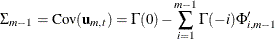
Partial Canonical Correlation Matrices

The partial canonical correlations at lag m between the vectors $\mb{y} _{t}$ and $\mb{y} _{t-m}$ , given $\mb{y} _{t-1}, \ldots , \mb{y} _{t-m+1}$ , are $1\geq \rho _1(m) \geq \rho _2(m) \cdots \geq \rho _ k(m)$ . The partial canonical correlations are the canonical correlations between the residual series $\mb{u} _{m,t}$ and $\mb{u} _{m,t-m}^{*}$ , where $\mb{u} _{m,t}$ and $\mb{u} _{m,t-m}^{*}$ are defined in the previous section. Thus, the squared partial canonical correlations $\rho _ i^2(m)$ are the eigenvalues of the matrix

$\{ \mr{Cov} (\mb{u} _{m,t})\} ^{-1} \mr{E} (\mb{u} _{m,t} \mb{u} _{m,t-m}^{*'}) \{ \mr{Cov} (\mb{u} _{m,t-m}^{*})\} ^{-1} \mr{E} (\mb{u} _{m,t-m}^{*} \mb{u} _{m,t}^{'}) = \Phi _{mm}^{*'} \Phi _{mm}^{'}$

It follows that the test statistic to test for $\Phi _ m = 0$ in the VAR model of order $m>p$ is approximately

$(T-m)\mr{~ tr~ } \{ \Phi _{mm}^{*'} \Phi _{mm}^{'} \} \approx (T-m)\sum _{i=1}^ k \rho _ i^2(m)$

and has an asymptotic chi-square distribution with $k^2$ degrees of freedom for $m>p$ .

The following statements use the PCANCORR option to compute the partial canonical correlations:

proc varmax data=simul1;
   model y1 y2 / p=1 noint lagmax=3 print=(pcancorr);
run;

Figure 42.57 shows that the partial canonical correlations $\rho _ i(m)$ between $\mb{y} _ t$ and $\mb{y} _{t-m}$ are {0.918, 0.773}, {0.092, 0.018}, and {0.109, 0.011} for lags $m=$ 1 to 3. After lag $m=$ 1, the partial canonical correlations are insignificant with respect to the 0.05 significance level, indicating that an AR order of $m=1$ can be an appropriate choice.

Figure 42.57: Partial Canonical Correlations (PCANCORR Option)

The VARMAX Procedure

Partial Canonical Correlations
Lag	Correlation1	Correlation2	DF	Chi-Square	Pr > ChiSq
1	0.91783	0.77335	4	142.61	<.0001
2	0.09171	0.01816	4	0.86	0.9307
3	0.10861	0.01078	4	1.16	0.8854

The Minimum Information Criterion (MINIC) Method

The minimum information criterion (MINIC) method can tentatively identify the orders of a VARMA(p,q) process (Spliid 1983; Koreisha and Pukkila 1989; Quinn 1980). The first step of this method is to obtain estimates of the innovations series, $\bepsilon _ t$ , from the VAR( $p_{\epsilon }$ ), where $p_{\epsilon }$ is chosen sufficiently large. The choice of the autoregressive order, $p_{\epsilon }$ , is determined by use of a selection criterion. From the selected VAR( $p_{\epsilon }$ ) model, you obtain estimates of residual series

$\tilde{ \bepsilon _ t} = \mb{y} _ t - \sum _{i=1}^{p_{\epsilon }} {\hat\Phi }_{i}^{p_{\epsilon }} \mb{y} _{t-i} - {\hat{\bdelta }}^{p_{\epsilon }}, ~ ~ t=p_{\epsilon }+1, \ldots , T$

In the second step, you select the order ( $p,q$ ) of the VARMA model for p in $(p_{min}:p_{max})$ and q in $(q_{min}:q_{max})$

$\mb{y} _ t = \bdelta + \sum _{i=1}^{p}{\Phi _{i}}\mb{y} _{t-i} - \sum _{i=1}^{q}{\Theta _{i}} \tilde{\bepsilon }_{t-i} + {\bepsilon _ t}$

which minimizes a selection criterion like SBC or HQ.

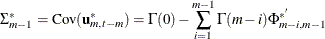
According to Lütkepohl (1993), the information criteria, namely Akaike’s information criterion (AIC), the corrected Akaike’s information criterion (AICC), the final prediction error criterion (FPE), the Hannan-Quinn criterion (HQC), and the Schwarz Bayesian criterion (SBC), are defined as

$\begin{eqnarray*} \mbox{AIC} & = & \log (|\tilde{\Sigma }|) + 2r_ b k/T \\ \mbox{AICC}& = & \log (|\tilde{\Sigma }|) + 2r_ b k/(T-r_ b) \\ \mbox{FPE} & = & (\frac{T+r_ b}{T-r_ b})^{k}|\tilde{\Sigma }| \\ \mbox{HQC} & = & \log (|\tilde{\Sigma }|) + 2r_ b k\log (\log (T))/T \\ \mbox{SBC} & = & \log (|\tilde{\Sigma }|) + r_ b k\log (T)/T \end{eqnarray*}$

where $\tilde{\Sigma }$ is the maximum likelihood estimate of the innovation covariance matrix $\Sigma$ , $r_ b$ is the number of parameters in each mean equation, k is the number of dependent variables, and T is the number of observations used to estimate the model. Compared to the definitions of AIC, AICC, HQC, and SBC discussed in the section Multivariate Model Diagnostic Checks, the preceding definitions omit some constant terms and are normalized by T. More specifically, only the parameters in each of the mean equations are counted; the parameters in the innovation covariance matrix $\Sigma$ are not counted.

The following statements use the MINIC= option to compute a table that contains the information criterion associated with various AR and MA orders:

proc varmax data=simul1;
   model y1 y2 / p=1 noint minic=(p=3 q=3);
run;

Figure 42.58 shows the output associated with the MINIC= option. The criterion takes the smallest value at AR order 1.

Figure 42.58: MINIC= Option

The VARMAX Procedure

Minimum Information Criterion Based on AICC
Lag	MA 0	MA 1	MA 2	MA 3
AR 0	3.3574947	3.0331352	2.7080996	2.3049869
AR 1	0.5544431	0.6146887	0.6771732	0.7517968
AR 2	0.6369334	0.6729736	0.7610413	0.8481559
AR 3	0.7235629	0.7551756	0.8053765	0.8654079