The QLIM Procedure
- Overview
-
Getting Started

-
Syntax
-
DetailsOrdinal Discrete Choice ModelingLimited Dependent Variable ModelsStochastic Frontier Production and Cost ModelsHeteroscedasticity and Box-Cox TransformationBivariate Limited Dependent Variable ModelingSelection ModelsMultivariate Limited Dependent ModelsVariable SelectionTests on ParametersEndogeneity and Instrumental VariablesPanel Data AnalysisBayesian AnalysisPrior DistributionsAutomated MCMCMarginal LikelihoodStandard DistributionsOutput to SAS Data SetOUTEST= Data SetNamingODS Table NamesODS Graphics
-
Examples
- References
Introductory Example: Binary Probit and Logit Models
The following example illustrates the use of PROC QLIM. The data were originally published by Mroz (1987) and downloaded from Wooldridge (2002). This data set is based on a sample of 753 married white women. The dependent variable is a discrete variable of labor force
participation (inlf ). Explanatory variables are the number of children ages 5 or younger (kidslt6 ), the number of children ages 6 to 18 (kidsge6 ), the woman’s age (age ), the woman’s years of schooling (educ ), wife’s labor experience (exper ), square of experience (expersq ), and the family income excluding the wife’s wage (nwifeinc ). The program (with data values omitted) is as follows:
/*-- Binary Probit --*/
proc qlim data=mroz plots=predicted;
   model inlf = nwifeinc educ exper expersq
                age kidslt6 kidsge6  / discrete;
run;
Results of this analysis are shown in the following four figures. In the first table, shown in Figure 29.1, PROC QLIM provides frequency information about each choice. In this example, 428 women participate in the labor force (inlf =1).
Figure 29.1: Choice Frequency Summary
The second table is the estimation summary table shown in Figure 29.2. Included are the number of dependent variables, names of dependent variables, the number of observations, the log-likelihood function value, the maximum absolute gradient, the number of iterations, AIC, and Schwarz criterion.
Figure 29.2: Fit Summary Table of Binary Probit
Goodness-of-fit measures are displayed in Figure 29.3. All measures except McKelvey-Zavoina’s definition are based on the log-likelihood function value. The likelihood ratio test
statistic has chi-square distribution conditional on the null hypothesis that all slope coefficients are zero. In this example,
the likelihood ratio statistic is used to test the hypothesis that kidslt6 =kidge6 =age =educ =exper =expersq 
nwifeinc = 0.
Figure 29.3: Goodness of Fit
| Goodness-of-Fit Measures | ||
|---|---|---|
| Measure | Value | Formula |
| Likelihood Ratio (R) | 227.14 | 2 * (LogL - LogL0) |
| Upper Bound of R (U) | 1029.7 | - 2 * LogL0 |
| Aldrich-Nelson | 0.2317 | R / (R+N) |
| Cragg-Uhler 1 | 0.2604 | 1 - exp(-R/N) |
| Cragg-Uhler 2 | 0.3494 | (1-exp(-R/N)) / (1-exp(-U/N)) |
| Estrella | 0.2888 | 1 - (1-R/U)^(U/N) |
| Adjusted Estrella | 0.2693 | 1 - ((LogL-K)/LogL0)^(-2/N*LogL0) |
| McFadden's LRI | 0.2206 | R / U |
| Veall-Zimmermann | 0.4012 | (R * (U+N)) / (U * (R+N)) |
| McKelvey-Zavoina | 0.4025 | |
| N = # of observations, K = # of regressors | ||
The parameter estimates and standard errors are shown in Figure 29.4.
Figure 29.4: Parameter Estimates of Binary Probit
| Parameter Estimates | |||||
|---|---|---|---|---|---|
| Parameter | DF | Estimate | Standard Error |
t Value | Approx Pr > |t| |
| Intercept | 1 | 0.270077 | 0.508590 | 0.53 | 0.5954 |
| nwifeinc | 1 | -0.012024 | 0.004840 | -2.48 | 0.0130 |
| educ | 1 | 0.130905 | 0.025255 | 5.18 | <.0001 |
| exper | 1 | 0.123348 | 0.018720 | 6.59 | <.0001 |
| expersq | 1 | -0.001887 | 0.000600 | -3.14 | 0.0017 |
| age | 1 | -0.052853 | 0.008477 | -6.24 | <.0001 |
| kidslt6 | 1 | -0.868329 | 0.118519 | -7.33 | <.0001 |
| kidsge6 | 1 | 0.036005 | 0.043477 | 0.83 | 0.4076 |
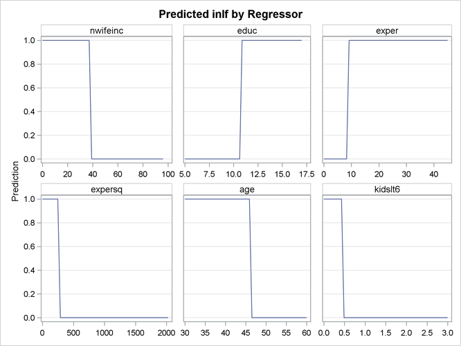
Finally, the QLIM procedure profiles the predicted outcome with respect to the regressors. For example, Figure 29.5 shows the predicted values profiled with respect to nwifeinc, educ, exper, expersq, age, and kidslt6.
Figure 29.5: Predictions by Regressors: nwifeinc, educ, exper, expersq, age, and kidslt6
When the error term has a logistic distribution, the binary logit model is estimated. To specify a logistic distribution, add D=LOGIT option as follows:
/*-- Binary Logit --*/
proc qlim data=mroz;
   model inlf = nwifeinc educ exper expersq
                age kidslt6 kidsge6  / discrete(d=logit);
run;
The estimated parameters are shown in Figure 29.6.
Figure 29.6: Parameter Estimates of Binary Logit
| Binary Data |
| Parameter Estimates | |||||
|---|---|---|---|---|---|
| Parameter | DF | Estimate | Standard Error |
t Value | Approx Pr > |t| |
| Intercept | 1 | 0.425452 | 0.860365 | 0.49 | 0.6210 |
| nwifeinc | 1 | -0.021345 | 0.008421 | -2.53 | 0.0113 |
| educ | 1 | 0.221170 | 0.043441 | 5.09 | <.0001 |
| exper | 1 | 0.205870 | 0.032070 | 6.42 | <.0001 |
| expersq | 1 | -0.003154 | 0.001017 | -3.10 | 0.0019 |
| age | 1 | -0.088024 | 0.014572 | -6.04 | <.0001 |
| kidslt6 | 1 | -1.443354 | 0.203575 | -7.09 | <.0001 |
| kidsge6 | 1 | 0.060112 | 0.074791 | 0.80 | 0.4215 |
The heteroscedastic logit model can be estimated using the HETERO statement. If the variance of the logit model is a function
of the family income level excluding wife’s income (nwifeinc ), the variance can be specified as
![\[ \hbox{Var}(\epsilon _{i}) = \sigma ^2 \, \exp (\gamma \hbox{*nwifeinc}_{i}) \]](images/etsug_qlim0002.png)
where  is normalized to 1 because the dependent variable is discrete. The following SAS statements estimate the heteroscedastic
logit model:
is normalized to 1 because the dependent variable is discrete. The following SAS statements estimate the heteroscedastic
logit model:
/*-- Binary Logit with Heteroscedasticity --*/
proc qlim data=mroz;
  model inlf = nwifeinc educ exper expersq
               age kidslt6 kidsge6 / discrete(d=logit);
  hetero inlf ~ nwifeinc / noconst;
run;
The parameter estimate,  , of the heteroscedasticity variable is listed as
 _H.nwifeinc; see Figure 29.7.
Figure 29.7: Parameter Estimates of Binary Logit with Heteroscedasticity
| Binary Data |
| Parameter Estimates | |||||
|---|---|---|---|---|---|
| Parameter | DF | Estimate | Standard Error |
t Value | Approx Pr > |t| |
| Intercept | 1 | 0.510445 | 0.983538 | 0.52 | 0.6038 |
| nwifeinc | 1 | -0.026778 | 0.012108 | -2.21 | 0.0270 |
| educ | 1 | 0.255547 | 0.061728 | 4.14 | <.0001 |
| exper | 1 | 0.234105 | 0.046639 | 5.02 | <.0001 |
| expersq | 1 | -0.003613 | 0.001236 | -2.92 | 0.0035 |
| age | 1 | -0.100878 | 0.021491 | -4.69 | <.0001 |
| kidslt6 | 1 | -1.645206 | 0.311296 | -5.29 | <.0001 |
| kidsge6 | 1 | 0.066941 | 0.085633 | 0.78 | 0.4344 |
| _H.nwifeinc | 1 | 0.013280 | 0.013606 | 0.98 | 0.3291 |