The QLIM Procedure
- Overview
-
Getting Started

-
Syntax
-
DetailsOrdinal Discrete Choice ModelingLimited Dependent Variable ModelsStochastic Frontier Production and Cost ModelsHeteroscedasticity and Box-Cox TransformationBivariate Limited Dependent Variable ModelingSelection ModelsMultivariate Limited Dependent ModelsVariable SelectionTests on ParametersEndogeneity and Instrumental VariablesPanel Data AnalysisBayesian AnalysisPrior DistributionsAutomated MCMCMarginal LikelihoodStandard DistributionsOutput to SAS Data SetOUTEST= Data SetNamingODS Table NamesODS Graphics
-
Examples
- References
Marginal Likelihood
The Bayes theorem states that
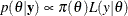
where  is a vector of parameters and
  is the product of the prior densities that are specified in the PRIOR
statement. The term
is the product of the prior densities that are specified in the PRIOR
statement. The term  is the likelihood that is associated with the MODEL
statement. The function
is the likelihood that is associated with the MODEL
statement. The function  is the nonnormalized posterior distribution over the parameter vector . The normalized posterior distribution (simply, the posterior distribution) is
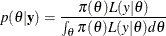
The denominator 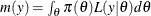 (also called the “marginal likelihood”) is a quantity of interest because it represents the probability of the data after
the effect of the parameter vector has been averaged out. Because of its interpretation, the marginal likelihood can be used
in various applications, including model averaging, variable selection, and model selection.
(also called the “marginal likelihood”) is a quantity of interest because it represents the probability of the data after
the effect of the parameter vector has been averaged out. Because of its interpretation, the marginal likelihood can be used
in various applications, including model averaging, variable selection, and model selection.
A natural estimate of the marginal likelihood is provided by the harmonic mean,
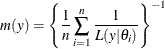
where  is a sample draw from the posterior distribution. In practical applications, this estimator has proven to be unstable.
An alternative and more stable estimator can be obtained with an importance sampling scheme. The auxiliary distribution for the importance sampler can be chosen through the cross entropy theory (Chan and Eisenstat 2015). In particular, given a parametric family of distributions, the auxiliary density function is chosen to be the one closest, in terms of the Kullback-Leibler divergence, to the probability density that would give a zero variance estimate of the marginal likelihood. In practical terms, this is equivalent to the following algorithm:
-
Choose a parametric family,
 , for the parameters of the model:
  .
.
-
Evaluate the maximum likelihood estimator of
 by using the posterior samples
  as data.
-
Use
 to generate the importance samples
  .
.
-
Estimate the marginal likelihood:
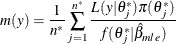
The parametric family for the auxiliary distribution is chosen to be Gaussian. The parameters that are subject to bounds are transformed accordingly
-
If
 , then
  .
.
-
If
 , then
  .
.
-
If
 , then
  .
.
-
If
 , then
  .
.
Assuming independence for the parameters that are subject to bounds, the auxiliary distribution to generate importance samples is
![\begin{equation*} \begin{pmatrix} \mb{p} \\ \mb{q} \\ \mb{r} \\ \mb{s} \end{pmatrix} \sim \mb{N} \left[ \begin{pmatrix} \mu _ p \\ \mu _{q} \\ \mu _{r} \\ \mu _{s} \\ \end{pmatrix}, \begin{pmatrix} \Sigma _ p & 0 & 0 & 0 \\ 0 & \Sigma _ q & 0 & 0 \\ 0 & 0 & \Sigma _ r & 0 \\ 0 & 0 & 0 & \Sigma _ r \\ \end{pmatrix} \right] \end{equation*}](images/etsug_qlim0464.png)
where  ,
,  ,
,  , and
, and  are vectors that contain the transformations of the unbounded, bounded-below, bounded-above, and bounded-above-and-below
parameters. Also, given the imposed independence structure,
are vectors that contain the transformations of the unbounded, bounded-below, bounded-above, and bounded-above-and-below
parameters. Also, given the imposed independence structure,  can be a nondiagonal matrix, but
  ,
,  , and
, and  are assumed to be diagonal matrices.