The QLIM Procedure
- Overview
-
Getting Started

-
Syntax
-
DetailsOrdinal Discrete Choice ModelingLimited Dependent Variable ModelsStochastic Frontier Production and Cost ModelsHeteroscedasticity and Box-Cox TransformationBivariate Limited Dependent Variable ModelingSelection ModelsMultivariate Limited Dependent ModelsVariable SelectionTests on ParametersEndogeneity and Instrumental VariablesPanel Data AnalysisBayesian AnalysisPrior DistributionsAutomated MCMCMarginal LikelihoodStandard DistributionsOutput to SAS Data SetOUTEST= Data SetNamingODS Table NamesODS Graphics
-
Examples
- References
Automated MCMC
The main purpose is to provide the user with the opportunity of obtaining a good approximation of the posterior distribution without initializing the MCMC algorithm: initial values, proposal distributions, burn-in and number of samples.
The automated algorithm is composed of two phases: tuning and sampling. In the tuning phase, there are two main concerns: the choice of a good proposal distribution and the search for the stationary region of the posterior distribution. In the sampling phase, the algorithm will decide how many samples are necessary to obtain good approximations of the posterior mean and some quantiles of interest.
Stationarity Phase
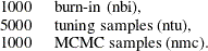
During the stationarity phase, the algorithm tries to search for a good proposal distribution and, at the same time, to reach the stationary region of the posterior. The choice of the proposal distribution is based on the analysis of the acceptance rates. This is similar to what is done in PROC MCMC: for more details see Tuning the Proposal Distribution: Tuning the Proposal Distribution in SAS/STAT 14.1 User's Guide. For the stationarity analysis, the main idea is to run two tests, Geweke (Ge) and Heidleberger-Welch (HW), on the posterior chains at the end of each attempt. For more details, see Geweke Diagnostics: Geweke Diagnostics in SAS/STAT 14.1 User's Guide, and Heidelberger and Welch Diagnostics: Heidelberger and Welch Diagnostics in SAS/STAT 14.1 User's Guide. If the stationarity hypothesis is rejected, then the tuning samples are increased and the tests repeated in the next attempt. After 10 attempts, the stationarity phase will be ended regardless of the results. The tuning parameters for the first attempt are fixed:
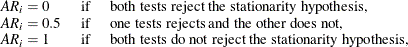
For the remaining attempts, the tuning parameters will be adjusted dynamically. More specifically, each parameter will be assigned an acceptance ratio (AR) of the stationarity hypothesis:
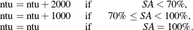
for  . For the Geweke test, the implemented significance level is 0.05. Then, an overall stationarity average (
 ) for all parameters ratios is evaluated,

and the number of tuning samples is updated accordingly:
The Heidelberger-Welch test also provides an indications of how much burn-in should be used. The algorithm requires this burn-in
to be:  . If that is not the case, the burn-in will updated accordingly,
 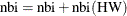 , and a new attempt searching for stationarity will be implemented. This choice is motivated by the fact that the burn-in
must be discarded in order to reach the stationary region of the posterior distribution.
, and a new attempt searching for stationarity will be implemented. This choice is motivated by the fact that the burn-in
must be discarded in order to reach the stationary region of the posterior distribution.
The number of samples is updated at each attempt. However, in order to exit the stationarity phase, it will not be required
 . The default update is
  . Depending on the outcome of the Raftery-Lewis diagnostics, if
 ![$\text {nmc}<\min \left\{ \text {LB}\left[\text {nmc}(\text {RL})\right],\text {nmc}(\text {RL})\right\} $](images/etsug_qlim0434.png) , the number of sampling is further updated to
, the number of sampling is further updated to ![$\text {nmc}= \text {LB}\left[\text {nmc}(\text {RL})\right]$](images/etsug_qlim0435.png) . By default,
. By default, ![$\text {LB}\left[\text {nmc}(\text {RL})\right]=10000$](images/etsug_qlim0436.png) . Finally, if the number of projected samples is not sufficient to perform a stable evaluation of the Raftery-Lewis test,
the number of samples is updated to
. Finally, if the number of projected samples is not sufficient to perform a stable evaluation of the Raftery-Lewis test,
the number of samples is updated to ![$\text {nmc}= \min \left[\text {nmc}(\text {RL})\right]$](images/etsug_qlim0437.png) . For more details see AUTOMCMC <phrase remap="Optional">=(<phrase remap="Argument">automcmc-options</phrase>)</phrase> and Raftery and Lewis Diagnostics: Raftery and Lewis Diagnostics in SAS/STAT 14.1 User's Guide.
. For more details see AUTOMCMC <phrase remap="Optional">=(<phrase remap="Argument">automcmc-options</phrase>)</phrase> and Raftery and Lewis Diagnostics: Raftery and Lewis Diagnostics in SAS/STAT 14.1 User's Guide.
Accuracy Phase
The main idea of the accuracy phase is to make sure that the mean and a quantile of interest are evaluated accurately. This can be tested by implementing the half-width test by Heidelberger-Welch and by analyzing the Raftery-Lewis diagnostic tool. In addition, the requirements defined in the stationarity phase will also be checked: the Geweke and the Heidelberger-Welch tests must not reject the stationary hypothesis and the burn-in predicted by the Heidelberger-Welch test must be zero.
The accuracy phase is characterized by a maximum of 10 attempts. If the algorithm exceeds this limit, the accuracy phase will
end and indications on how to improve sampling will be given. The search of accuracy can be performed using two different
method. The first method (the default) is triggered by the option TARGETSTATS and it is based on the accuracy analysis of
the mean and a percentile of interest. The secong method is triggered by the option TARGETESS and it targets a minimum number
of effective samples. The accuracy phase will first update the burn-in with the information provided by the HW test: . Then, it determines the difference between the actual number of samples and the number of samples predicted by either the
RL test or the ESS: ![$\Delta [\text {nmc}]=\text {nmc}(\text {RL})-\text {nmc},$](images/etsug_qlim0438.png) or
or ![$\Delta [\text {nmc}]=\text {nmc}(\text {ESS})-\text {nmc}.$](images/etsug_qlim0439.png) The new number of samples will be updated accordingly:
The new number of samples will be updated accordingly:
![\begin{equation*} \begin{tabular}{lll} $\text {nmc}=\text {nmc}+\text {LB}\left[\text {nmc}(\text {RL})\right]$ & if & \qquad \qquad \quad \, \, $0<\Delta [\text {nmc}]\leq \text {LB}\left[\text {nmc}(\text {RL})\right],$ \\ $\text {nmc}=\text {nmc}+\Delta [\text {nmc}]$ & if & $\text {LB}\left[\text {nmc}(\text {RL})\right]<\Delta [\text {nmc}]\leq \text {UB}\left[\text {nmc}(\text {RL})\right],$ \\ $\text {nmc}=\text {nmc}+\text {UB}\left[\text {nmc}(\text {RL})\right]$ & if & $\text {UB}\left[\text {nmc}(\text {RL})\right]<\Delta [\text {nmc}].$ \end{tabular}\end{equation*}](images/etsug_qlim0440.png)
By default, and ![$\text {UB}\left[\text {nmc}(\text {RL})\right]=300000$](images/etsug_qlim0441.png) .
.
In addition, the accuracy search triggered by the option TARGETSTATS also implements the HW half-width test to checks whether
the sample mean is accurate. If the mean of any parameters is not considered to be accurate and the number of samples has
not been updated based on ![$\Delta [\text {nmc}]$](images/etsug_qlim0442.png) , then the number of samples is increased:
, then the number of samples is increased:
![\begin{equation*} \begin{tabular}{lll} $\text {nmc}=\text {nmc}+5000$ & if & $\Delta [\text {nmc}]\leq 0$, \\ \end{tabular}\end{equation*}](images/etsug_qlim0443.png)