The PANEL Procedure
- Overview
- Getting Started
-
Syntax

-
DetailsSpecifying the Input DataSpecifying the Regression ModelUnbalanced DataMissing ValuesComputational ResourcesRestricted EstimatesNotationOne-Way Fixed-Effects ModelTwo-Way Fixed-Effects ModelBalanced PanelsUnbalanced PanelsFirst-Differenced Methods for One-Way and Two-Way ModelsBetween EstimatorsPooled EstimatorOne-Way Random-Effects ModelTwo-Way Random-Effects ModelHausman-Taylor EstimationAmemiya-MaCurdy EstimationParks Method (Autoregressive Model)Da Silva Method (Variance-Component Moving Average Model)Dynamic Panel EstimatorsLinear Hypothesis TestingHeteroscedasticity-Corrected Covariance MatricesHeteroscedasticity- and Autocorrelation-Consistent Covariance MatricesR-SquareSpecification TestsPanel Data Poolability TestPanel Data Cross-Sectional Dependence TestPanel Data Unit Root TestsLagrange Multiplier (LM) Tests for Cross-Sectional and Time EffectsTests for Serial Correlation and Cross-Sectional EffectsTroubleshootingCreating ODS GraphicsOUTPUT OUT= Data SetOUTEST= Data SetOUTTRANS= Data SetPrinted OutputODS Table Names
-
Examples
- References
Tests for Serial Correlation and Cross-Sectional Effects
- Baltagi and Li Joint LM Test for Serial Correlation and Random Cross-Sectional Effects
- Wooldridge Test for the Presence of Unobserved Effects
- Bera, Sosa Escudero, and Yoon Modified Rao’s Score Test in the Presence of Local Misspecification
- Baltagi and Li (1995) LM Test for First-Order Correlation under Fixed Effects
- Durbin-Watson Statistic
- Berenblut-Webb Statistic
- Testing for Random Walk Null Hypothesis
The presence of cross-sectional effects causes serial correlation in the errors. Therefore, serial correlation is often tested jointly with cross-sectional effects. Joint and conditional tests for both serial correlation and cross-sectional effects have been covered extensively in the literature.
Baltagi and Li Joint LM Test for Serial Correlation and Random Cross-Sectional Effects
Baltagi and Li (1991) derive the LM test statistic, which jointly tests for zero first-order serial correlation and random cross-sectional effects
under normality and homoscedasticity. The test statistic is independent of the form of serial correlation, so it can be used
with either AR or MA error terms. The null hypothesis is a white noise component:
 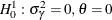 for MA with MA coefficient
  or
or 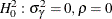 for AR with AR coefficient
  . The alternative is either a one-way random-effects model (cross-sectional) or first-order serial correlation AR or MA in errors or both. Under the null hypothesis, the model can be estimated by the pooled estimation (OLS). Denote the residuals
as
. The alternative is either a one-way random-effects model (cross-sectional) or first-order serial correlation AR or MA in errors or both. Under the null hypothesis, the model can be estimated by the pooled estimation (OLS). Denote the residuals
as  . The test statistic is
![\begin{equation*} \mr{BL91} = \frac{NT^{2}}{2\left(T-1\right)\left(T-2\right)}\left[A^{2}-4AB+2TB^{2}\right]\xrightarrow {H_{0}^{1,2}}\chi ^{2}\left(2\right) \end{equation*}](images/etsug_panel1053.png)
where
Wooldridge Test for the Presence of Unobserved Effects
Wooldridge (2002, sec. 10.4.4) suggests a test for the absence of an unobserved effect. Under the null hypothesis  , the errors
  are serially uncorrelated. To test , Wooldridge (2002) proposes to test for AR(1) serial correlation. The test statistic that he proposes is
![\begin{equation*} W = \frac{\sum _{i = 1}^{N}\sum _{t = 1}^{T-1}\sum _{s = t + 1}^{T}\hat{u}_{it}\hat{u}_{is}}{\left[\sum _{i = 1}^{N}\left(\sum _{t = 1}^{T-1}\sum _{s = t + 1}^{T}\hat{u}_{it}\hat{u}_{is}\right)^{2}\right]^{1/2}}\rightarrow \mathcal{N}\left(0,1\right) \end{equation*}](images/etsug_panel1056.png)
where are the pooled OLS residuals. The test statistic W can detect many types of serial correlation in the error term u, so it has power against both the one-way random-effects specification and the serial correlation in error terms.
Bera, Sosa Escudero, and Yoon Modified Rao’s Score Test in the Presence of Local Misspecification
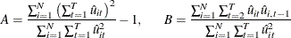
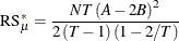
Bera, Sosa Escudero, and Yoon (2001) point out that the standard specification tests, such as the Honda (1985) test described in the section Honda (1985) and Honda (1991) UMP Test and Moulton and Randolph (1989) SLM Test, are not valid when they test for either cross-sectional random effects or serial correlation without considering the presence of the other effects. They suggest a modified Rao’s score (RS) test. When A and B are defined as in Baltagi and Li (1991) , the test statistic for testing serial correlation under random cross-sectional effects is
Baltagi and Li (1991, 1995) derive the conventional RS test when the cross-sectional random effects is assumed to be absent:

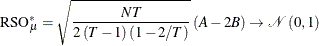
Symmetrically, to test for the cross-sectional random effects in the presence of serial correlation, the modified Rao’s score test statistic is
and the conventional Rao’s score test statistic is given in Breusch and Pagan (1980). The test statistics are asymptotically distributed as  .
.
Because  , the one-sided test is expected to lead to more powerful tests. The one-sided test can be derived by taking the signed square
root of the two-sided statistics:
, the one-sided test is expected to lead to more powerful tests. The one-sided test can be derived by taking the signed square
root of the two-sided statistics:
Baltagi and Li (1995) LM Test for First-Order Correlation under Fixed Effects
The two-sided LM test statistic for testing a white noise component in a fixed one-way model ( or
or  , given that
  are fixed effects) is
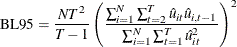
where are the residuals from the fixed one-way model (FIXONE). The LM test statistic is asymptotically distributed as  under the null hypothesis. The one-sided LM test with alternative hypothesis
  is
is
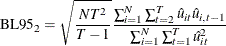
which is asymptotically distributed as standard normal.
Durbin-Watson Statistic
Bhargava, Franzini, and Narendranathan (1982) propose a test of the null hypothesis of no serial correlation () against the alternative ( ) by the Durbin-Watson statistic,
where are the residuals from the fixed one-way model (FIXONE).
The test statistic  is a locally most powerful invariant test in the neighborhood of
  . Some of the upper and lower bounds are listed in Bhargava, Franzini, and Narendranathan (1982). To test against a positive correlation (
 ) for very large N, you can simply detect whether
  . However, for small-to-moderate N, the mechanics of the Durbin-Watson test produce a region of uncertainty as to whether to reject the null hypothesis. The
output contains two p-values: The first, Pr < DWLower, treats the uncertainty region as a rejection region. The second, Pr > DWUpper, is more conservative
and treats the uncertainty region as a failure-to-reject region. You can think of these two p-values as bounds on the exact p-value.
. However, for small-to-moderate N, the mechanics of the Durbin-Watson test produce a region of uncertainty as to whether to reject the null hypothesis. The
output contains two p-values: The first, Pr < DWLower, treats the uncertainty region as a rejection region. The second, Pr > DWUpper, is more conservative
and treats the uncertainty region as a failure-to-reject region. You can think of these two p-values as bounds on the exact p-value.
Berenblut-Webb Statistic
Bhargava, Franzini, and Narendranathan (1982) suggest using the Berenblut-Webb statistic, which is a locally most powerful invariant test in the neighborhood of  . The test statistic is
where  are the residuals from the first-difference estimation. The upper and lower bounds are the same as for the Durbin-Watson
statistic and produce two p-values, one conservative and one anti-conservative.
are the residuals from the first-difference estimation. The upper and lower bounds are the same as for the Durbin-Watson
statistic and produce two p-values, one conservative and one anti-conservative.
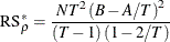
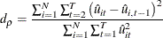
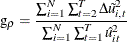
Testing for Random Walk Null Hypothesis
You can also use the Durbin-Watson and Berenblut-Webb statistics to test the random walk null hypothesis, with the bounds
that are listed in Bhargava, Franzini, and Narendranathan (1982). For more information about these statistics, see the sections Durbin-Watson Statistic and Berenblut-Webb Statistic. Bhargava, Franzini, and Narendranathan (1982) also propose the R statistic to test the random walk null hypothesis against the stationary alternative
  . Let
. Let  , where
  is a
is a  symmetric matrix that has the following elements:

The test statistic is
![\begin{equation*} \begin{array}{l l l} \mr{R}_{\rho } & = & \Delta \tilde{U}’\Delta \tilde{U}/\Delta \tilde{U}’F^{*} \Delta \tilde{U}\\ & = & \frac{\sum _{i=1}^{N}\sum _{t=2}^{T}\Delta \tilde{u}_{i,t}^{2}}{\left[\sum _{i=1}^{N}\sum _{t=2}^{T}\left(t-1\right) \left(T-t+1\right)\Delta \tilde{u}_{i,t}^{2}+2 \sum _{i=1}^{N}\sum _{t=2}^{T-1}\sum _{t'=t+1}^{T} \left(T-t'+1\right)\left(t-1\right)\Delta \tilde{u}_{i,t}\Delta \tilde{u}_{i,t'}\right]/T} \end{array}\end{equation*}](images/etsug_panel1083.png)
The statistics R, g, and d can be used with the same bounds. They satisfy  , and they are equivalent for large panels.