The PANEL Procedure
- Overview
- Getting Started
-
Syntax

-
DetailsSpecifying the Input DataSpecifying the Regression ModelUnbalanced DataMissing ValuesComputational ResourcesRestricted EstimatesNotationOne-Way Fixed-Effects ModelTwo-Way Fixed-Effects ModelBalanced PanelsUnbalanced PanelsFirst-Differenced Methods for One-Way and Two-Way ModelsBetween EstimatorsPooled EstimatorOne-Way Random-Effects ModelTwo-Way Random-Effects ModelHausman-Taylor EstimationAmemiya-MaCurdy EstimationParks Method (Autoregressive Model)Da Silva Method (Variance-Component Moving Average Model)Dynamic Panel EstimatorsLinear Hypothesis TestingHeteroscedasticity-Corrected Covariance MatricesHeteroscedasticity- and Autocorrelation-Consistent Covariance MatricesR-SquareSpecification TestsPanel Data Poolability TestPanel Data Cross-Sectional Dependence TestPanel Data Unit Root TestsLagrange Multiplier (LM) Tests for Cross-Sectional and Time EffectsTests for Serial Correlation and Cross-Sectional EffectsTroubleshootingCreating ODS GraphicsOUTPUT OUT= Data SetOUTEST= Data SetOUTTRANS= Data SetPrinted OutputODS Table Names
-
Examples
- References
Heteroscedasticity- and Autocorrelation-Consistent Covariance Matrices
The HAC option in the MODEL statement selects the type of heteroscedasticity- and autocorrelation-consistent covariance matrix.
As with the HCCME option, an estimator of the middle expression  in sandwich form is needed. With the HAC option, it is estimated as
![\[ \Lambda _{\mr{HAC}}=a\sum _{i = 1} ^{N} \sum _{t=1}^{T_ i} \hat{\epsilon }_{it} ^{2}\mb{x} _{it} \mb{x} _{it} ^{'} +a\sum _{i = 1} ^{N} \sum _{t=1}^{T_ i} \sum _{s=1}^{t-1} k(\frac{s-t}{b})\hat{\epsilon }_{it}\hat{\epsilon }_{is}\left(\mb{x} _{it} \mb{x} _{is} ^{'}+\mb{x} _{is} \mb{x} _{it} ^{'}\right) \]](images/etsug_panel0666.png)
, where  is the real-valued kernel function[6], b is the bandwidth parameter, and a is the adjustment factor of small sample degrees of freedom (that is,
  if the ADJUSTDF option is not specified and otherwise
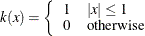
  , where k is the number of parameters including dummy variables). The types of kernel functions are listed in Table 27.2.
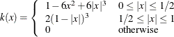
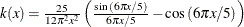
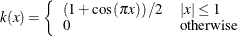
Table 27.2: Kernel Functions
|
Kernel Name |
Equation |
|---|---|
|
Bartlett |
|
|
Parzen |
|
|
Quadratic spectral |
|
|
Truncated |
|
|
Tukey-Hanning |
|
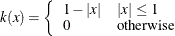
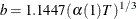
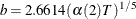
When the BANDWIDTH=ANDREWS option is specified, the bandwidth parameter is estimated as shown in Table 27.3.
Table 27.3: Bandwidth Parameter Estimation
|
Kernel Name |
Bandwidth Parameter |
|---|---|
|
Bartlett |
|
|
Parzen |
|
|
Quadratic spectral |
|
|
Truncated |
|
|
Tukey-Hanning |
|
Let  denote each series in
  , and let
  denote the corresponding estimates of the autoregressive and innovation variance parameters of the AR(1) model on ,
  , where the AR(1) model is parameterized as
 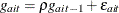 with
with  . The
. The  and
and  are estimated with the following formulas:
![\[ \alpha (1) = \frac{\sum _{a=1}^ k{\frac{4\rho _ a^{2}\sigma _ a^4}{(1-\rho _ a)^6(1+\rho _ a)^2}}}{\sum _{a=1}^ k{\frac{\sigma _ a^4}{(1-\rho _ a)^4}}} \\ \alpha (2) = \frac{\sum _{a=1}^ k{\frac{4\rho _ a^{2}\sigma _ a^4}{(1-\rho _ a)^8}}}{\sum _{a=1}^ k{\frac{\sigma _ a^4}{(1-\rho _ a)^4}}} \]](images/etsug_panel0689.png)
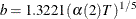
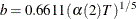
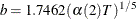
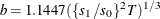
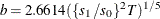
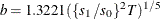
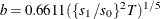
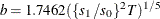
When you specify BANDWIDTH=NEWEYWEST94, according to Newey and West (1994) the bandwidth parameter is estimated as shown in Table 27.4.
Table 27.4: Bandwidth Parameter Estimation
|
Kernel Name |
Bandwidth Parameter |
|---|---|
|
Bartlett |
|
|
Parzen |
|
|
Quadratic spectral |
|
|
Truncated |
|
|
Tukey-Hanning |
|
The  and
and  are estimated with the following formulas:
![\[ s_1 = 2\sum _{j=1}^ n{j\sigma _ j} \\ s_0 = \sigma _0+2\sum _{j=1}^ n{\sigma _ j} \]](images/etsug_panel0697.png)
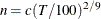
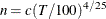
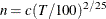
where n is the lag selection parameter and is determined by kernels, as listed in Table 27.5.
Table 27.5: Lag Selection Parameter Estimation
|
Kernel Name |
Lag Selection Parameter |
|---|---|
|
Bartlett |
|
|
Parzen |
|
|
Quadratic Spectral |
|
|
Truncated |
|
|
Tukey-Hanning |
|
The c in Table 27.5 is specified by the C= option; by default, C=12.
The  is estimated with the equation
![\[ \sigma _ j = T^{-1}\sum _{t=j+1}^{T}{\left(\sum _{a=i}^ k{g_{at}}\sum _{a=i}^ k{g_{at-j}}\right)}, j=0, ..., n \]](images/etsug_panel0703.png)
where  is the same as in the Andrews method and i is 1 if the NOINT option in the MODEL statement is specified, and 2 otherwise.
When you specify BANDWIDTH=SAMPLESIZE, the bandwidth parameter is estimated with the equation
![\[ b = \left\{ \begin{array}{ l l } \left\lfloor {\gamma T^{r} + c} \right\rfloor & \text {if BANDWIDTH=SAMPLESIZE(INT) option is specified} \\ \gamma T^{r} + c & \text {otherwise} \end{array} \right. \]](images/etsug_panel0705.png)
where T is the sample size,  is the largest integer less than or equal to x, and
  , r, and c are values specified by BANDWIDTH=SAMPLESIZE(GAMMA=, RATE=, CONSTANT=) options, respectively.
If the PREWHITENING option is specified in the MODEL statement,  is prewhitened by the VAR(1) model,
![\[ g_{it} = A_{i} g_{i,t-1} + w_{it} \]](images/etsug_panel0708.png)
Then  is calculated by
![\[ \Lambda _{\mr{HAC}}=a\sum _{i = 1} ^{N}\left\{ \left(\sum _{t=1}^{T_{i}}{w_{it} w_{it}’}+\sum _{t=1}^{T_{i}}{\sum _{s=1}^{t-1}{k(\frac{s-t}{b})\left(w_{it} w_{is}’ + w_{is} w_{it}’\right)}}\right)(I-A_{i})^{-1}((I-A_{i})^{-1})’\right\} \]](images/etsug_panel0710.png)
