Hypothesis Testing and Estimation :: SAS/STAT(R) 14.1 User's Guide

Degrees of Freedom

In this section, degrees of freedom (df) refers to the denominator degrees of freedom for F statistics in hypothesis testing. It also refers to the degrees of freedom in t tests for parameter estimates and odds ratio estimates, and for computing t distribution percentiles for confidence limits of these estimates. The value of df is determined by the design degrees of freedom f and by what you specify in the DF= option in the MODEL statement.

The default df is determined as

$df=\left\{ { \begin{array}{ll} ~ f-r+1 & \mbox{for Taylor variance estimation method} \\ ~ f & \mbox{for replication variance estimation methods} \end{array}} \right.$

where f is the design degrees of freedom and r is the rank of the contrast of model parameters to be tested.

Design Degrees of Freedom f

The design degrees of freedom f is determined by the survey design and the variance estimation method.

Design Degrees of Freedom f for the Taylor Series Method

For Taylor series variance estimation, the design degrees of freedom f can depend on the number of clusters, the number of strata, and the number of observations. These numbers are based on the observations that are included in the analysis; they do not count observations that are excluded from the analysis because of missing values. If all values in a stratum are excluded from the analysis as missing values, then that stratum is called an empty stratum. Empty strata are not counted in the total number of strata for the analysis. Similarly, empty clusters and missing observations are not included in the totals counts of clusters and observations that are used to compute the f for the analysis.

If you specify the MISSING option in the CLASS statement, missing values are treated as valid nonmissing levels and are included in determining the f. If you specify the NOMCAR option for Taylor series variance estimation, observations that have missing values for variables in the regression model are included. For more information about missing values, see the section Missing Values.

Using the notation that is defined in the section Notation, let $\tilde n$ be the total number of clusters if the design has a CLUSTER statement; let n be the total sample size; and let H be the number of strata if there is a STRATA statement, or 1 otherwise. Then for Taylor series variance estimation, the design degrees of freedom is

$f=\left\{ { \begin{array}{ll}/* */ \tilde n - H & \mbox{if the design contains clusters} \\ n - H & \mbox{if the design does not contain clusters} \end{array}} \right.$

Design Degrees of Freedom f for the Replication Method

For the replication variance estimation method, the design degrees of freedom f depends on the replication method that you use or whether you use replication weights.

If you provide replicate weights but you do not specify DF=value in the REPWEIGHTS statement, f is the number of replicates.
If you specify the DF=value option in a REPWEIGHTS statement, then f=value.
If you do not provide replicate weights and use BRR (including Fay’s method ) method, then f=H, which is the number of strata.
If you do not provide replicate weights and use the jackknife method, then $f=R-H$ , where R is the number of replicates and H is the number of strata if you specify a STRATA statement or H = 1 otherwise.

Setting Design Degrees of Freedom f to a Specific Value

If you do not want to use the default design degrees of freedom, then you can specify the DF=DESIGN(value) or DF=PARMADJ(value) (for Taylor method only) option in the MODEL statement, where value is a positive number. Then f=value.

However, if you specify the value in the DF= option in the MODEL statement as well as with the DF= option in a REPWEIGHTS statement, then the df is determined by the value in the MODEL statement, and the DF= option in the REPWEIGHTS statement is ignored.

Setting Design Degrees of Freedom to Infinity

If you specify DF=INFINITY in the MODEL statement, then the df is set to be infinite.

As the denominator degrees of freedom grows, an F distribution approaches a chi-square distribution, and similarly a t distribution approaches a normal distribution. Therefore, when you specify DF=INFINITY in the MODEL statement), PROC SURVEYLOGISTIC uses chi-square tests and normal distribution percentiles to construct confidence intervals.

Modifying Degrees of Freedom with the Number of Parameters

When you use Taylor series variance estimation (by default or when you specify VARMETHOD=TAYLOR in the MODEL statement), and you are fitting a model that has many parameters relative to the design degrees of freedom, it is appropriate to modify the design degrees of freedom by using the number of nonsingular parameters p in the model (Korn and Graubard (1999, section 5.2), Rao, Scott, and Skinner (1998)). You can specify DF=PARMADJ or DF=PARMADJ(value) in the MODEL statement to request this modification only for Taylor series variance estimation method; and this option does not apply to the replication variance estimation method.

Let f be the design degrees of freedom that is described in the section Design Degrees of Freedom f for the Taylor Series Method. By default, or if you specify the DF=PARMADJ option, the df is modified as $df=f-p+1$ .

Testing Global Null Hypothesis: BETA=0

The global null hypothesis refers to the null hypothesis that all the explanatory effects can be eliminated and the model can contain only intercepts. By using the notations in the section Logistic Regression Models, the global null hypothesis is defined as follows:

If you have a cumulative model whose model parameters are $\btheta = (\balpha ’,\bbeta ’)’$ , where $\balpha$ are the parameters for the intercepts and $\bbeta$ are the parameters for the explanatory effects, then $H_0: \bbeta =\Strong{0}$ . The number of restrictions r that are imposed on $\btheta$ is the number of parameters in slope parameter $\bbeta =(\beta _{1}, \beta _{2}, \ldots , \beta _{k})’$ : $r=k$ .
If you have a generalized logit model whose model parameters are $\btheta = ( \bbeta _1’, \bbeta _2’, \ldots , \bbeta _ D’)’$ and $\bbeta _ d = (\beta _{d1}, \beta _{d2}, \ldots , \beta _{dk})’ \, \, \, (d=1, 2, \ldots , D)$ , then $H_0: (\beta _{d2}, \ldots , \beta _{dk})’=\Strong{0} \, \, \, (d=1, 2, \ldots , D)$ . The number of restrictions r that are imposed on $\btheta$ is the total number of slope parameters in $\bbeta _1’, \bbeta _2’, \ldots , \bbeta _ D’$ : $r=(k-1)*D$ .

PROC SURVEYLOGISTIC displays these tests in the "Testing Global Null Hypothesis: BETA=0" table.

Rao-Scott Likelihood Ratio Chi-Square Test

For complex survey design, you can use a design-adjusted Rao-Scott likelihood ratio chi-square test to test the global null hypothesis. For information about design-adjusted chi-square tests, see Lohr (2010, Section 10.3.2), Rao and Scott (1981), Rao and Scott (1984), Rao and Scott (1987), Thomas and Rao (1987), Rao and Thomas (1989), and Thomas, Singh, and Roberts (1996).

If you specify the CHISQ(NOADJUST) option, PROC SURVEYLOGISTIC computes the likelihood ratio chi-square test without the Rao-Scott design correction. If you specify the CHISQ(FIRSTORDER) option, PROC SURVEYLOGISTIC performs a first-order Rao-Scott likelihood ratio chi-square test. If you specify the CHISQ(SECONDORDER) option, PROC SURVEYLOGISTIC performs a second-order Rao-Scott likelihood ratio chi-square test.

If you do not specify the CHISQ option, the default test depends on the design and the model. By default, PROC SURVEYLOGISTIC performs a first-order or second-order Rao-Scott likelihood ratio chi-square (Satterthwaite) test if your design is not simple random sampling or when you provide replicate weights. Otherwise, if your design is simple random sampling and you do not provide replicate weights, PROC SURVEYLOGISTIC does not make any adjustment for the likelihood ratio test. In other words:

If your design does not contain stratification nor clustering, and you do not provide replicate weights, then by default PROC SURVEYLOGISTIC performs a likelihood ratio chi-square test without any adjustment.
If your design contains either stratification or clustering, or if you provide replicate weights, then by default PROC SURVEYLOGISTIC performs a likelihood ratio chi-square test with Rao-Scott adjustment. However, the default order of the adjustment depends on the number of model parameters excluding the intercepts.
- If there is more than one nonintercept parameter in the model, the default is the second-order Rao-Scott likelihood ratio test.
- If there is only one nonintercept parameter in the model, there is no need to compute the second-order adjustment. Therefore, the default is the first-order Rao-Scott likelihood ratio test.

Let $\hat{\btheta }$ be the estimated parameters, let $\hat{\btheta }_{H_0}$ be the estimated parameters under the global null hypothesis, and let r be the restrictions imposed on $\btheta$ under the global null hypothesis $H_0$ . Let $L(\btheta )$ be the log-likelihood function.

Denote the estimated covariance matrix of $\hat{\btheta }$ under simple random sampling as $\hat V^{\mbox{srs}}(\hat{\btheta })$ , and its partition corresponding to the r slope parameters as ${\hat V^{\mbox{srs}}_{rr}}(\hat{\btheta })$ . Similarly, denote the estimated covariance matrix of $\hat{\btheta }$ under the sample design as $\hat V(\hat{\btheta })$ , and its partition corresponding to the r slope parameters as $\hat V_{rr}(\hat{\btheta })$ .

Define the design effect matrix E as

$E=\hat V_{rr}(\hat{\btheta }) \left({\hat V^{\mbox{srs}}_{rr}}(\hat{\btheta })\right)^{-1}$

Denote $r^*$ as the rank of E and the positive eigenvalues of the design matrix E as $\delta _1 \ge \delta _2 \ge \cdots \ge \delta _{r^*} > 0$ .

Likelihood Ratio Chi-Square Test

Without the Rao-Scott design correction, the global null hypothesis is tested using either the chi-square statistics,

$Q_{\chi ^{2}}= 2 \left[ L (\hat{\btheta }) - L(\hat{\btheta }_{H_0}) \right]$

with r degrees of freedom, or an equivalent F statistics,

$F= 2 \left[ L (\hat{\btheta }) - L(\hat{\btheta }_{H_0}) \right] / r$

with $(r,\infty )$ degrees of freedom.

Rao-Scott First-Order Chi-Square Test

To address the impact of a complex survey design on the significance level of the likelihood ratio test, Rao and Scott (1984) proposed a first-order correction to the chi-square statistics as

$Q_{RS1}=Q_{\chi ^{2}}/\bar\delta _\cdot$

where the first-order design correction,

$\bar\delta _\cdot = \sum _{i=1}^{r^*} {\delta _ i}/r^*$

is the average of positive eigenvalues of the design effect matrix E.

Under the null hypothesis, the first-order Rao-Scott chi-square $Q_{RS1}$ approximately follows a chi-square distribution with $r^*$ degrees of freedom.

The corresponding F statistic is

$F_{RS1} = Q_{RS1} / r^*$

which has an F distribution with $r^*$ and $df{\cdot }r^*$ degrees of freedom under the null hypothesis (Thomas and Rao 1984, 1987), and df is the design degrees of freedom as described in the section Design Degrees of Freedom f for the Taylor Series Method.

Rao-Scott Second-Order Chi-Square Test

Rao and Scott (1987) further proposed the second-order (Satterthwaite) Rao-Scott chi-square statistic as

$Q_{RS2}=Q_{RS1}/(1 + \hat a^2)$

where $Q_{RS1}$ is the first-order Rao-Scott chi-square statistic and the second-order design correction is computed from the coefficient of variation of the eigenvalues of the design effect matrix E as

$\hat a^2=\frac{1}{r^*-1}\sum _{i=1}^{r^*} {(\delta _ i-\bar\delta _\cdot )^2} / {\bar\delta _\cdot ^2}$

Under the null hypothesis, the second-order Rao-Scott chi-square $Q_{RS2}$ approximately follows a chi-square distribution with $r^*/(1+\hat{a}^2)$ degrees of freedom.

The corresponding F statistic is

$F_{RS2} = Q_{RS2} (1+\hat{a}^2) / r^*$

which has an F distribution with $r^*/(1+\hat{a}^2)$ and $df{\cdot }r^*/(1+\hat{a}^2)$ degrees of freedom under the null hypothesis (Thomas and Rao 1984, 1987), and df is the design degrees of freedom as described in the section Design Degrees of Freedom f for the Taylor Series Method.

Score Statistics and Tests

To express the general form of the score statistic, let $\btheta$ be the parameter vector you want to estimate and let ${\mb{g}}(\btheta )$ be the vector of first partial derivatives (gradient vector) of the log likelihood with respect to the parameter vector $\btheta$ .

Consider a null hypothesis $H_0$ that has r restrictions imposed on $\btheta$ . Let $\hat{\btheta }$ be the MLE of $\btheta$ under $H_0$ , let $\mb{g}(\hat{\btheta })$ be the gradient vector evaluated at $\hat{\btheta }$ , and let ${\hat{\mb{V}}}(\hat{\btheta })$ be the estimated covariance matrix for $\hat{\btheta }$ , which is described in the section Variance Estimation.

For the Taylor series variance estimation method, by default (or when DF=PARMADJ ), PROC SURVEYLOGISTIC computes the score test statistic for the null hypothesis $H_0$ as

$W_{F}=\left( \frac{f-r+1}{f \, \, r} \right) \mb{g}(\hat{\btheta })’ \left[{\hat{\mb{V}}}(\hat{\btheta }) \right]^{-1} \mb{g}(\hat{\btheta })$

where f is the design degrees of freedom as described in the section Design Degrees of Freedom f for the Taylor Series Method.

If you specify DF=DESIGN option or if you use the replication variance estimation method, PROC SURVEYLOGISTIC computes the score test statistic for the null hypothesis $H_0$ as

$W_{F}= \frac{1}{r} \mb{g}(\hat{\btheta })’ \left[{\hat{\mb{V}}}(\hat{\btheta }) \right]^{-1} \mb{g}(\hat{\btheta })$

Under $H_0$ , $W_{F}$ has an F distribution with $(r,df)$ degrees of freedom, where the denominator degrees of freedom df is described in the section Degrees of Freedom.

As the denominator degrees of freedom grows, an F distribution approaches a chi-square distribution, and similarly a t distribution approaches a normal distribution. If you specify DF=INFINITY in the MODEL statement, the score test statistic for both Taylor series and replication methods for testing the null hypothesis $H_0$ can be expressed as

$W_{\chi ^{2}}=\mb{g}(\hat{\btheta })’\left[{\hat{\mb{V}}}(\hat{\btheta }) \right]^{-1} \mb{g}(\hat{\btheta })$

$W_{\chi ^{2}}$ has a chi-square distribution with r degrees of freedom under the null hypothesis $H_0$ .

Testing the Parallel Lines Assumption

For a model that has an ordinal response, the parallel lines assumption depends on the link function, which you can specify in the LINK= option in the MODEL statement. When the link function is probit or complementary log-log, the parallel lines assumption is the equal slopes assumption; PROC SURVEYLOGISTIC displays the corresponding test in the "Score Test for the Equal Slopes Assumption" table. When the link function is logit, the parallel lines assumption is the proportional odds assumption; PROC SURVEYLOGISTIC displays the corresponding test in the "Score Test for the Proportional Odds Assumption" table. This section describes the computation of the score tests of these assumptions.

For this test, the number of response levels, $D+1$ , is assumed to be strictly greater than 2. Let Y be the response variable taking values $1, \ldots , D, D+1$ . Suppose there are k explanatory variables. Consider the general cumulative model without making the parallel lines assumption:

$g(\mbox{Pr}(Y\leq d~ |~ \mb{x}))= (1,\mb{x})\btheta _ d, \quad 1 \leq d \leq D$

where $g(\cdot )$ is the link function, and ${\btheta }_ d=(\alpha _ d, \beta _{d1}, \ldots , \beta _{dk})^\prime$ is a vector of unknown parameters consisting of an intercept $\alpha _ d$ and k slope parameters $\beta _{k1}, \ldots , \beta _{kd}$ . The parameter vector for this general cumulative model is

$\btheta =(\btheta ’_1,\ldots ,\btheta ’_ D)’$

Under the null hypothesis of parallelism $H_0\colon \beta _{1i}=\beta _{2i}=\cdots =\beta _{Di}, 1 \leq i \leq k$ , there is a single common slope parameter for each of the k explanatory variables. Let $\beta _1,\dots ,\beta _ k$ be the common slope parameters. Let $\hat{\alpha }_1, \ldots , \hat{\alpha }_ D$ and $\hat{\beta }_1, \ldots , \hat{\beta }_ D$ be the MLEs of the intercept parameters and the common slope parameters. Then, under $H_0$ , the MLE of $\btheta$ is

$\hat{\btheta }=(\hat{\btheta }’_1,\ldots ,\hat{\btheta }’_ D)’ \quad \mbox{with} \quad \hat{\btheta }_ d=(\hat{\alpha }_ d,\hat{\beta }_1,\ldots , \hat{\beta }_ k)’, \quad 1 \leq d \leq D$

and the chi-square score statistic 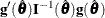${\mb{g}}’(\hat{\btheta })\mb{I}^{-1}(\hat{\btheta }){\mb{g}}(\hat{\btheta })$ has an asymptotic chi-square distribution with $k(D-1)$ degrees of freedom. This tests the parallel lines assumption by testing the equality of separate slope parameters simultaneously for all explanatory variables.

Note that this test is the same as what PROC LOGISTIC produces. It does not compute a score test that uses the covariance matrix incorporated with the survey design information as described in the section Score Statistics and Tests.

Wald Confidence Intervals for Parameters

Wald confidence intervals are sometimes called normal confidence intervals. They are based on the asymptotic normality of the parameter estimators. The $100(1-\alpha )$ % Wald confidence interval for $\theta _ j$ is given by

$\hat{\theta }_ j \pm z_{1-\alpha /2}\hat{\sigma }_ j$

where $z_{1-\alpha /2}$ is the $100(1-\alpha /2)$ th percentile of the standard normal distribution, $\hat{\theta }_ j$ is the pseudo-estimate of $\theta _ j$ , and $\hat{\sigma }_ j$ is the standard error estimate of $\hat{\theta }_ j$ in the section Variance Estimation.

Testing Linear Hypotheses about the Regression Coefficients

Linear hypotheses for $\btheta$ can be expressed in matrix form as

$H_0\colon \mb{L}\btheta = \mb{c}$

where $\mb{L}$ is a matrix of coefficients for the linear hypotheses and $\mb{c}$ is a vector of constants whose rank is r. The vector of regression coefficients $\btheta$ includes both slope parameters and intercept parameters.

Let $\hat{\btheta }$ be the MLE of $\btheta$ , and let $\hat{\bV }(\hat{\btheta })$ be the estimated covariance matrix that is described in the section Variance Estimation.

For the Taylor series variance estimation method, PROC SURVEYLOGISTIC computes the test statistic for the null hypothesis $H_0$ as

$W_{F}=\left( \frac{f-r+1}{f \, \, r} \right) (\mb{L}\hat{\btheta } - \mb{c})’ [{\mb{L}\hat{\bV }(\hat{\btheta })\mb{L}’}]^{-1} (\mb{L}\hat{\btheta } - \mb{c})$

where f is the design degrees of freedom as described in the section Design Degrees of Freedom f for the Taylor Series Method.

For the replication variance estimation method, PROC SURVEYLOGISTIC computes the test statistic for the null hypothesis $H_0$ as

$W_{F}= \frac{1}{r} (\mb{L}\hat{\btheta } - \mb{c})’ [{\mb{L}\hat{\bV }(\hat{\btheta })\mb{L}’}]^{-1} (\mb{L}\hat{\btheta } - \mb{c})$

Under the $H_0$ , $W_{F}$ has an F distribution with $(r,df)$ degrees of freedom, and the denominator degrees of freedom df is described in the section Degrees of Freedom.

As the denominator degrees of freedom grows, an F distribution approaches a chi-square distribution, and similarly a t distribution approaches a normal distribution. If you specify DF=INFINITY in the MODEL statement, PROC SURVEYLOGISTIC computes the test statistic for both Taylor series and replication methods for testing the null hypothesis $H_0$ as

$W_{\chi ^{2}} = (\mb{L}\hat{\btheta } - \mb{c})’ [{\mb{L}\hat{\bV }(\hat{\btheta })\mb{L}’}]^{-1} (\mb{L}\hat{\btheta } - \mb{c})$

Under $H_0$ , $\chi ^2_{W}$ has an asymptotic chi-square distribution with r degrees of freedom.

Type 3 Tests

For models that use less-than-full-rank parameterization (as specified by the PARAM=GLM option in the CLASS statement), a Type 3 test of an effect of interest (main effect or interaction) is a test of the Type III estimable functions that are defined for that effect. When the model contains no missing cells, the Type 3 test of a main effect corresponds to testing the hypothesis of equal marginal means. For more information about Type III estimable functions, see Chapter 46: The GLM Procedure, and Chapter 15: The Four Types of Estimable Functions. Also see Littell, Freund, and Spector (1991).

For models that use full-rank parameterization, all parameters are estimable when there are no missing cells, so it is unnecessary to define estimable functions. The standard test of an effect of interest in this case is the joint test that the values of the parameters associated with that effect are zero. For a model that uses effects parameterization (as specified by the PARAM=EFFECT option in the CLASS statement), the joint test for a main effect is equivalent to testing the equality of marginal means. For a model that uses reference parameterization (as specified by the PARAM=REF option in the CLASS statement), the joint test is equivalent to testing the equality of cell means at the reference level of the other model effects. For more information about the coding scheme and the associated interpretation of results, see Muller and Fetterman (2002, Chapter 14).

If there is no interaction term, the Type 3 test of an effect for a model that uses GLM parameterization is the same as the joint test of the effect for the model that uses full-rank parameterization. In this situation, the joint test is also called the Type 3 test. For a model that contains an interaction term and no missing cells, the Type 3 test of a component main effect under GLM parameterization is the same as the joint test of the component main effect under effect parameterization. Both test the equality of cell means. But this Type 3 test differs from the joint test under reference parameterization, which tests the equality of cell means at the reference level of the other component main effect. If some cells are missing, you can obtain meaningful tests only by testing a Type III estimation function, so in this case you should use GLM parameterization.

The results of a Type 3 test or a joint test do not depend on the order in which you specify the terms in the MODEL statement.

Odds Ratio Estimation

Consider a dichotomous response variable with outcomes event and nonevent. Let a dichotomous risk factor variable X take the value 1 if the risk factor is present and 0 if the risk factor is absent. According to the logistic model, the log odds function, $g(X)$ , is given by

$g(X) \equiv \log \biggl (\frac{\Pr (~ \mathit{event} ~ |~ X)}{\Pr (~ \mathit{nonevent} ~ |~ X)} \biggr ) = \beta _0 + \beta _1 X \\$

The odds ratio $\psi$ is defined as the ratio of the odds for those with the risk factor (X = 1) to the odds for those without the risk factor (X = 0). The log of the odds ratio is given by

$\log (\psi ) \equiv \log (\psi (X=1,X=0)) = g(X=1) - g(X=0) = \beta _1$

The parameter, $\beta _1$ , associated with X represents the change in the log odds from X = 0 to X = 1. So the odds ratio is obtained by simply exponentiating the value of the parameter associated with the risk factor. The odds ratio indicates how the odds of event change as you change X from 0 to 1. For instance, $\psi =2$ means that the odds of an event when X = 1 are twice the odds of an event when X = 0.

Suppose the values of the dichotomous risk factor are coded as constants a and b instead of 0 and 1. The odds when $X = a$ become $\exp (\beta _0 + a \beta _1)$ , and the odds when $X = b$ become $\exp (\beta _0 + b \beta _1)$ . The odds ratio corresponding to an increase in X from a to b is

$\psi = \exp [(b - a) \beta _1] = [\exp (\beta _1)]^{b-a} \equiv [\exp (\beta _1)]^ c$

Note that for any a and b such that $c=b-a=1, \psi =\exp (\beta _1)$ . So the odds ratio can be interpreted as the change in the odds for any increase of one unit in the corresponding risk factor. However, the change in odds for some amount other than one unit is often of greater interest. For example, a change of one pound in body weight might be too small to be considered important, while a change of 10 pounds might be more meaningful. The odds ratio for a change in X from a to b is estimated by raising the odds ratio estimate for a unit change in X to the power of $c=b-a$ , as shown previously.

For a polytomous risk factor, the computation of odds ratios depends on how the risk factor is parameterized. For illustration, suppose that Race is a risk factor with four categories: White, Black, Hispanic, and Other.

For the effect parameterization scheme (PARAM=EFFECT) with White as the reference group, the design variables for Race are as follows.

	Design Variables
Race	$X_1$	$X_2$	$X_3$
Black	1	0	0
Hispanic	0	1	0
Other	0	0	1
White	–1	–1	–1

The log odds for Black is

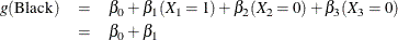
$\begin{eqnarray*} g(\textrm{Black}) & =& \beta _0 + \beta _1 (X_1=1) + \beta _2 (X_2=0) + \beta _3 (X_3=0) \\ & =& \beta _0 + \beta _1 \end{eqnarray*}$

The log odds for White is

$\begin{eqnarray*} g(\textrm{White}) & =& \beta _0 + \beta _1 (X_1=-1) + \beta _2 (X_2=-1)+ \beta _3 (X_3=-1)) \\ & =& \beta _0 - \beta _1 - \beta _2 - \beta _3 \end{eqnarray*}$

Therefore, the log odds ratio of Black versus White becomes

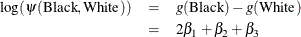
$\begin{eqnarray*} \log (\psi (\textrm{Black},\textrm{White})) & =& g(\textrm{Black}) - g(\textrm{White}) \\ & =& 2 \beta _1 + \beta _2 + \beta _3 \end{eqnarray*}$

For the reference cell parameterization scheme (PARAM=REF) with White as the reference cell, the design variables for race are as follows.

	Design Variables
Race	$X_1$	$X_2$	$X_3$
Black	1	0	0
Hispanic	0	1	0
Other	0	0	1
White	0	0	0

The log odds ratio of Black versus White is given by

$\begin{eqnarray*} {\log (\psi (\textrm{Black},\textrm{White}))} & = & g(\textrm{Black}) - g(\textrm{White}) \\ & = & (\beta _0 + \beta _1 (X_1=1) + \beta _2 (X_2=0)) + \beta _3 (X_3=0)) - \\ & & (\beta _0 + \beta _1 (X_1=0) + \beta _2 (X_2=0) + \beta _3 (X_3=0)) \\ & = & \beta _1 \end{eqnarray*}$

For the GLM parameterization scheme (PARAM=GLM), the design variables are as follows.

	Design Variables
Race	$X_1$	$X_2$	$X_3$	$X_4$
Black	1	0	0	0
Hispanic	0	1	0	0
Other	0	0	1	0
White	0	0	0	1

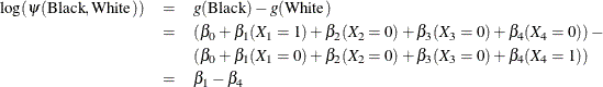
The log odds ratio of Black versus White is

$\begin{eqnarray*} {\log (\psi (\textrm{Black},\textrm{White}))} & = & g(\textrm{Black}) - g(\textrm{White}) \\ & = & (\beta _0 + \beta _1 (X_1=1) + \beta _2 (X_2=0) + \beta _3 (X_3=0) + \beta _4 (X_4=0)) -\\ & & (\beta _0 + \beta _1 (X_1=0) + \beta _2 (X_2=0) + \beta _3 (X_3=0) + \beta _4(X_4=1)) \\ & = & \beta _1 - \beta _4 \end{eqnarray*}$

Consider the hypothetical example of heart disease among race in Hosmer and Lemeshow (2000, p. 51). The entries in the following contingency table represent counts.

	Race
Disease Status	White	Black	Hispanic	Other
Present	5	20	15	10
Absent	20	10	10	10

The computation of odds ratio of Black versus White for various parameterization schemes is shown in Table 111.9.

Table 111.9: Odds Ratio of Heart Disease Comparing Black to White

	Parameter Estimates
PARAM=	$\hat{\beta _1}$	$\hat{\beta _2}$	$\hat{\beta _3}$	$\hat{\beta _4}$	Odds Ratio Estimates
EFFECT	0.7651	0.4774	0.0719		$\exp (2 \times 0.7651 + 0.4774 + 0.0719) = 8$
REF	2.0794	1.7917	1.3863		$\exp (2.0794) = 8$
GLM	2.0794	1.7917	1.3863	0.0000	$\exp (2.0794) = 8$

Since the log odds ratio ( $\log (\psi )$ ) is a linear function of the parameters, the Wald confidence interval for $\log (\psi )$ can be derived from the parameter estimates and the estimated covariance matrix. Confidence intervals for the odds ratios are obtained by exponentiating the corresponding confidence intervals for the log odd ratios. In the displayed output of PROC SURVEYLOGISTIC, the "Odds Ratio Estimates" table contains the odds ratio estimates and the corresponding t or Wald confidence intervals computed by using the covariance matrix in the section Variance Estimation. For continuous explanatory variables, these odds ratios correspond to a unit increase in the risk factors.

To customize odds ratios for specific units of change for a continuous risk factor, you can use the UNITS statement to specify a list of relevant units for each explanatory variable in the model. Estimates of these customized odds ratios are given in a separate table. Let $(L_ j,U_ j)$ be a confidence interval for $\log (\psi )$ . The corresponding lower and upper confidence limits for the customized odds ratio $\exp (c\beta _ j)$ are $\exp (cL_ j)$ and $\exp (cU_ j)$ , respectively, (for $c>0$ ); or $\exp (cU_ j)$ and $\exp (cL_ j)$ , respectively, (for c < 0). You use the CLODDS option in the MODEL statement to request confidence intervals for the odds ratios.

For a generalized logit model, odds ratios are computed similarly, except D odds ratios are computed for each effect, corresponding to the D logits in the model.

Rank Correlation of Observed Responses and Predicted Probabilities

The predicted mean score of an observation is the sum of the ordered values (shown in the "Response Profile" table) minus one, weighted by the corresponding predicted probabilities for that observation; that is, the predicted means score is $\sum _{d=1}^{D+1}(d-1)\hat{\pi }_ d$ , where D + 1 is the number of response levels and $\hat{\pi }_ d$ is the predicted probability of the dth (ordered) response.

A pair of observations with different observed responses is said to be concordant if the observation with the lower-ordered response value has a lower predicted mean score than the observation with the higher-ordered response value. If the observation with the lower-ordered response value has a higher predicted mean score than the observation with the higher-ordered response value, then the pair is discordant. If the pair is neither concordant nor discordant, it is a tie. Enumeration of the total numbers of concordant and discordant pairs is carried out by categorizing the predicted mean score into intervals of length $D / 500$ and accumulating the corresponding frequencies of observations.

Let N be the sum of observation frequencies in the data. Suppose there are a total of t pairs with different responses, $n_ c$ of them are concordant, $n_ d$ of them are discordant, and $t-n_ c-n_ d$ of them are tied. PROC SURVEYLOGISTIC computes the following four indices of rank correlation for assessing the predictive ability of a model:

$\begin{eqnarray*} & & c =(n_ c+0.5(t-n_ c-n_ d))/t \\ & & \mbox{Somers' } D =(n_ c-n_ d)/t \\ & & \mbox{Goodman-Kruskal gamma} =(n_ c-n_ d)/(n_ c+n_ d) \\ & & \mbox{Kendall's tau-}a =(n_ c-n_ d)/(0.5N(N-1)) \end{eqnarray*}$

Note that c also gives an estimate of the area under the receiver operating characteristic (ROC) curve when the response is binary (Hanley and McNeil 1982).

For binary responses, the predicted mean score is equal to the predicted probability for Ordered Value 2. As such, the preceding definition of concordance is consistent with the definition used in previous releases for the binary response model.

The SURVEYLOGISTIC Procedure