The SURVEYLOGISTIC Procedure
- Overview
- Getting Started
-
Syntax
 PROC SURVEYLOGISTIC StatementBY StatementCLASS StatementCLUSTER StatementCONTRAST StatementDOMAIN StatementEFFECT StatementESTIMATE StatementFREQ StatementLSMEANS StatementLSMESTIMATE StatementMODEL StatementOUTPUT StatementREPWEIGHTS StatementSLICE StatementSTORE StatementSTRATA StatementTEST StatementUNITS StatementWEIGHT Statement
 -
DetailsMissing ValuesModel SpecificationModel FittingSurvey Design InformationLogistic Regression Models and ParametersVariance EstimationDomain AnalysisHypothesis Testing and EstimationLinear Predictor, Predicted Probability, and Confidence LimitsOutput Data SetsDisplayed OutputODS Table NamesODS Graphics
-
Examples
- References
Logistic Regression Models and Parameters
The SURVEYLOGISTIC procedure fits a logistic regression model and estimates the corresponding regression parameters. Each model uses the link function you specified in the LINK= option in the MODEL statement. There are four types of model you can use with the procedure: cumulative logit model, complementary log-log model, probit model, and generalized logit model.
Notation
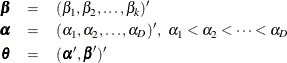
Let Y be the response variable with categories  . The p covariates are denoted by a p-dimension row vector
  .
.
For a stratified clustered sample design, each observation is represented by a row vector, 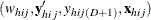 , where
-
 is the stratum index
-
 is the cluster index within stratum h
-
 is the unit index within cluster i of stratum h
-
 denotes the sampling weight
-
 is a D-dimensional column vector whose elements are indicator variables for the first D categories for variable Y. If the response of the jth unit of the ith cluster in stratum h falls in category d, the dth element of the vector is one, and the remaining elements of the vector are zero, where
  .
.
-
 is the indicator variable for the
  category of variable Y
-
 denotes the k-dimensional row vector of explanatory variables for the jth unit of the ith cluster in stratum h. If there is an intercept, then
  .
.
-
 is the total number of clusters in the sample
-
 is the total sample size
The following notations are also used:
-
 denotes the sampling rate for stratum h
-
 is the expected vector of the response variable:
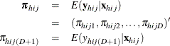
Note that  , where 1 is a D-dimensional column vector whose elements are 1.
Logistic Regression Models
If the response categories of the response variable Y can be restricted to a number of ordinal values, you can fit cumulative probabilities of the response categories with a cumulative
logit model, a complementary log-log model, or a probit model. Details of cumulative logit models (or proportional odds models)
can be found in McCullagh and Nelder (1989). If the response categories of Y are nominal responses without natural ordering, you can fit the response probabilities with a generalized logit model. Formulation
of the generalized logit models for nominal response variables can be found in Agresti (2002). For each model, the procedure estimates the model parameter  by using a pseudo-log-likelihood function. The procedure obtains the pseudo-maximum likelihood estimator
  by using iterations described in the section Iterative Algorithms for Model Fitting and estimates its variance described in the section Variance Estimation.
Cumulative Logit Model
A cumulative logit model uses the logit function
![\[ g(t)=\log \left( \frac{t}{1-t} \right) \]](images/statug_surveylogistic0191.png)
as the link function.
Denote the cumulative sum of the expected proportions for the first d categories of variable Y by
![\[ F_{hijd}=\sum _{r=1}^ d \pi _{hijr} \]](images/statug_surveylogistic0192.png)
for  Then the cumulative logit model can be written as
![\[ \log \left(\frac{F_{hijd}}{1-F_{hijd}}\right) = \alpha _ d+\mb{x}_{hij}\bbeta \]](images/statug_surveylogistic0194.png)
with the model parameters
Complementary Log-Log Model
A complementary log-log model uses the complementary log-log function
![\[ g(t)=\log (-\log (1-t)) \]](images/statug_surveylogistic0196.png)
as the link function. Denote the cumulative sum of the expected proportions for the first d categories of variable Y by
for Then the complementary log-log model can be written as
![\[ \log (-\log (1-F_{hijd}))=\alpha _ d+\mb{x}_{hij}\bbeta \]](images/statug_surveylogistic0197.png)
with the model parameters
Probit Model
A probit model uses the probit (or normit) function, which is the inverse of the cumulative standard normal distribution function,
![\[ g(t)=\Phi ^{-1}(t) \]](images/statug_surveylogistic0198.png)
as the link function, where
![\[ \Phi (t)=\frac{1}{\sqrt {2\pi }}\int _{-\infty }^ t e^{-\frac{1}{2} z^2} dz \]](images/statug_surveylogistic0199.png)
Denote the cumulative sum of the expected proportions for the first d categories of variable Y by
for Then the probit model can be written as
![\[ F_{hijd}=\Phi (\alpha _ d+\mb{x}_{hij}\bbeta ) \]](images/statug_surveylogistic0200.png)
with the model parameters
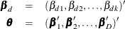
Generalized Logit Model
For nominal response, a generalized logit model is to fit the ratio of the expected proportion for each response category over the expected proportion of a reference category with a logit link function.
Without loss of generality, let category  be the reference category for the response variable Y. Denote the expected proportion for the dth category by
  as in the section Notation. Then the generalized logit model can be written as
![\[ \log \left(\frac{\pi _{hijd}}{\pi _{hij(D+1)}}\right) =\mb{x}_{hij}\bbeta _ d \]](images/statug_surveylogistic0202.png)
for  with the model parameters
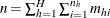
Likelihood Function
Let  be a link function such that
![\[ \bpi =\mb{g}(\mb{x}, \btheta ) \]](images/statug_surveylogistic0206.png)
where is a column vector for regression coefficients. The pseudo-log likelihood is
![\[ l(\btheta ) = \sum _{h=1}^ H\sum _{i=1}^{n_ h} \sum _{j=1}^{m_{hi}} w_{hij} \left( (\log (\bpi _{hij}))’\mb{y}_{hij}+ \log (\pi _{hij(D+1)})y_{hij(D+1)} \right) \]](images/statug_surveylogistic0207.png)
Denote the pseudo-estimator as , which is a solution to the estimating equations:
![\[ \sum _{h=1}^ H\sum _{i=1}^{n_ h} \sum _{j=1}^{m_{hi}} w_{hij}\mb{D}_{hij} \left(\mr{diag}(\bpi _{hij})-\bpi _{hij}\bpi _{hij}’\right)^{-1} (\mb{y}_{hij}-\bpi _{hij})= \Strong{0} \]](images/statug_surveylogistic0208.png)
where  is the matrix of partial derivatives of the link function
  with respect to .
To obtain the pseudo-estimator , the procedure uses iterations with a starting value  for . See the section Iterative Algorithms for Model Fitting for more details.