The SURVEYLOGISTIC Procedure
- Overview
- Getting Started
-
Syntax
 PROC SURVEYLOGISTIC StatementBY StatementCLASS StatementCLUSTER StatementCONTRAST StatementDOMAIN StatementEFFECT StatementESTIMATE StatementFREQ StatementLSMEANS StatementLSMESTIMATE StatementMODEL StatementOUTPUT StatementREPWEIGHTS StatementSLICE StatementSTORE StatementSTRATA StatementTEST StatementUNITS StatementWEIGHT Statement
 -
DetailsMissing ValuesModel SpecificationModel FittingSurvey Design InformationLogistic Regression Models and ParametersVariance EstimationDomain AnalysisHypothesis Testing and EstimationLinear Predictor, Predicted Probability, and Confidence LimitsOutput Data SetsDisplayed OutputODS Table NamesODS Graphics
-
Examples
- References
Model Fitting
Determining Observations for Likelihood Contributions
If you use the events/trials syntax, each observation is split into two observations. One has the response value 1 with a frequency equal to the value of the events variable. The other observation has the response value 2 and a frequency equal to the value of (trials – events). These two observations have the same explanatory variable values and the same WEIGHT values as the original observation.
For either the single-trial or the events/trials syntax, let j index all observations. In other words, for the single-trial syntax, j indexes the actual observations. And, for the events/trials syntax, j indexes the observations after splitting (as described previously). If your data set has 30 observations and you use the single-trial syntax, j has values from 1 to 30; if you use the events/trials syntax, j has values from 1 to 60.
Suppose the response variable in a cumulative response model can take on the ordered values  , where k is an integer
  . The likelihood for the jth observation with ordered response value
  and explanatory variables vector ( row vectors)
  is given by
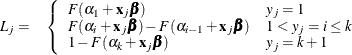
where  is the logistic, normal, or extreme-value distribution function;
  are ordered intercept parameters; and
  is the slope parameter vector.
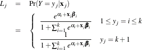
For the generalized logit model, letting the  st level be the reference level, the intercepts are unordered and the slope vector
  varies with each logit. The likelihood for the jth observation with ordered response value and explanatory variables vector (row vectors) is given by
Iterative Algorithms for Model Fitting
Two iterative maximum likelihood algorithms are available in PROC SURVEYLOGISTIC to obtain the pseudo-estimate  of the model parameter
  . The default is the Fisher scoring method, which is equivalent to fitting by iteratively reweighted least squares. The alternative
algorithm is the Newton-Raphson method. Both algorithms give the same parameter estimates; the covariance matrix of is estimated in the section Variance Estimation. For a generalized logit model, only the Newton-Raphson technique is available. You can use the TECHNIQUE=
option in the MODEL statement to select a fitting algorithm.
. The default is the Fisher scoring method, which is equivalent to fitting by iteratively reweighted least squares. The alternative
algorithm is the Newton-Raphson method. Both algorithms give the same parameter estimates; the covariance matrix of is estimated in the section Variance Estimation. For a generalized logit model, only the Newton-Raphson technique is available. You can use the TECHNIQUE=
option in the MODEL statement to select a fitting algorithm.
Iteratively Reweighted Least Squares Algorithm (Fisher Scoring)
Let Y be the response variable that takes values 
 . Let j index all observations and
  be the value of response for the jth observation. Consider the multinomial variable
 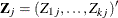 such that
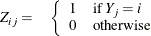
and  . With
  denoting the probability that the jth observation has response value i, the expected value of
  is
is  , and
, and  . The covariance matrix of is
  , which is the covariance matrix of a multinomial random variable for one trial with parameter vector
  . Let be the vector of regression parameters—for example,
  for cumulative logit model. Let
  be the matrix of partial derivatives of with respect to . The estimating equation for the regression parameters is
![\[ \sum _ j\mb{D}’_ j\mb{W}_ j(\mb{Z}_ j-\bpi _ j)=\mb{0} \]](images/statug_surveylogistic0139.png)
where  , and
, and  and
and  are the WEIGHT and FREQ values of the jth observation.
With a starting value of  , the pseudo-estimate of is obtained iteratively as
![\[ \btheta ^{(i+1)}=\btheta ^{(i)}+(\sum _ j \mb{D}’_ j\mb{W}_ j\mb{D}_ j)^{-1} \sum _ j\mb{D}’_ j\mb{W}_ j(\mb{Z}_ j-\bpi _ j) \]](images/statug_surveylogistic0144.png)
where ,  , and are evaluated at the ith iteration
  . The expression after the plus sign is the step size. If the log likelihood evaluated at
  is less than that evaluated at , then is recomputed by step-halving or ridging. The iterative scheme continues until convergence is obtained—that is, until is sufficiently close to . Then the maximum likelihood estimate of is
  .
.
By default, starting values are zero for the slope parameters, and starting values are the observed cumulative logits (that is, logits of the observed cumulative proportions of response) for the intercept parameters. Alternatively, the starting values can be specified with the INEST= option in the PROC SURVEYLOGISTIC statement.
Newton-Raphson Algorithm
Let
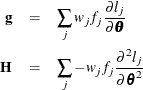
be the gradient vector and the Hessian matrix, where  is the log likelihood for the jth observation. With a starting value of , the pseudo-estimate of is obtained iteratively until convergence is obtained:
![\[ \btheta ^{(i+1)}=\btheta ^{(i)} +\mb{H}^{-1}\mb{g} \]](images/statug_surveylogistic0151.png)
where  and
and  are evaluated at the ith iteration . If the log likelihood evaluated at is less than that evaluated at , then is recomputed by step-halving or ridging. The iterative scheme continues until convergence is obtained—that is, until is sufficiently close to . Then the maximum likelihood estimate of is .
Convergence Criteria
Four convergence criteria are allowed: ABSFCONV= , FCONV= , GCONV= , and XCONV= . If you specify more than one convergence criterion, the optimization is terminated as soon as one of the criteria is satisfied. If none of the criteria is specified, the default is GCONV=1E–8.
Existence of Maximum Likelihood Estimates
The likelihood equation for a logistic regression model does not always have a finite solution. Sometimes there is a nonunique maximum on the boundary of the parameter space, at infinity. The existence, finiteness, and uniqueness of pseudo-estimates for the logistic regression model depend on the patterns of data points in the observation space (Albert and Anderson 1984; Santner and Duffy 1986).
Consider a binary response model. Let be the response of the ith subject, and let be the row vector of explanatory variables (including the constant 1 associated with the intercept). There are three mutually
exclusive and exhaustive types of data configurations: complete separation, quasi-complete separation, and overlap.
- Complete separation
-
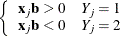
There is a complete separation of data points if there exists a vector
 that correctly allocates all observations to their response groups; that is,
This configuration gives nonunique infinite estimates. If the iterative process of maximizing the likelihood function is allowed to continue, the log likelihood diminishes to zero, and the dispersion matrix becomes unbounded.
- Quasi-complete separation
-
The data are not completely separable, but there is a vector
such that
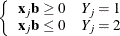
and equality holds for at least one subject in each response group. This configuration also yields nonunique infinite estimates. If the iterative process of maximizing the likelihood function is allowed to continue, the dispersion matrix becomes unbounded and the log likelihood diminishes to a nonzero constant.
- Overlap
-
If neither complete nor quasi-complete separation exists in the sample points, there is an overlap of sample points. In this configuration, the pseudo-estimates exist and are unique.
Complete separation and quasi-complete separation are problems typically encountered with small data sets. Although complete separation can occur with any type of data, quasi-complete separation is not likely with truly continuous explanatory variables.
The SURVEYLOGISTIC procedure uses a simple empirical approach to recognize the data configurations that lead to infinite parameter
estimates. The basis of this approach is that any convergence method of maximizing the log likelihood must yield a solution
that gives complete separation, if such a solution exists. In maximizing the log likelihood, there is no checking for complete
or quasi-complete separation if convergence is attained in eight or fewer iterations. Subsequent to the eighth iteration,
the probability of the observed response is computed for each observation. If the probability of the observed response is
one for all observations, there is a complete separation of data points and the iteration process is stopped. If the complete
separation of data has not been determined and an observation is identified to have an extremely large probability ( 0.95) of the observed response, there are two possible situations. First, there is overlap in the data set, and the observation
is an atypical observation of its own group. The iterative process, if allowed to continue, stops when a maximum is reached.
Second, there is quasi-complete separation in the data set, and the asymptotic dispersion matrix is unbounded. If any of the
diagonal elements of the dispersion matrix for the standardized observations vectors (all explanatory variables standardized
to zero mean and unit variance) exceeds 5,000, quasi-complete separation is declared and the iterative process is stopped.
If either complete separation or quasi-complete separation is detected, a warning message is displayed in the procedure output.
0.95) of the observed response, there are two possible situations. First, there is overlap in the data set, and the observation
is an atypical observation of its own group. The iterative process, if allowed to continue, stops when a maximum is reached.
Second, there is quasi-complete separation in the data set, and the asymptotic dispersion matrix is unbounded. If any of the
diagonal elements of the dispersion matrix for the standardized observations vectors (all explanatory variables standardized
to zero mean and unit variance) exceeds 5,000, quasi-complete separation is declared and the iterative process is stopped.
If either complete separation or quasi-complete separation is detected, a warning message is displayed in the procedure output.
Checking for quasi-complete separation is less foolproof than checking for complete separation. The NOCHECK option in the MODEL statement turns off the process of checking for infinite parameter estimates. In cases of complete or quasi-complete separation, turning off the checking process typically results in the procedure failing to converge.
Model Fitting Statistics
Suppose the model contains s explanatory effects. For the jth observation, let  be the estimated probability of the observed response. The three criteria displayed by the SURVEYLOGISTIC procedure are calculated
as follows:
be the estimated probability of the observed response. The three criteria displayed by the SURVEYLOGISTIC procedure are calculated
as follows:
-
–2 log likelihood:
![\[ -2\mbox{ Log L}=-2\sum _ j w_ j f_ j\log (\hat{\pi }_ j) \]](images/statug_surveylogistic0159.png)
where
and are the weight and frequency values, respectively, of the jth observation. For binary response models that use the events/trials syntax, this is equivalent to
![\[ -2\mbox{ Log L}=-2\sum _ j w_ j f_ j \{ r_ j \log (\hat{\pi }_ j) + (n_ j-r_ j)\log (1-\hat{\pi }_ j) \} \]](images/statug_surveylogistic0160.png)
where
 is the number of events,
  is the number of trials, and is the estimated event probability.
-
Akaike information criterion:
![\[ \mbox{AIC}=-2\mbox{ Log L}+2p \]](images/statug_surveylogistic0163.png)
where p is the number of parameters in the model. For cumulative response models,
 , where k is the total number of response levels minus one, and s is the number of explanatory effects. For the generalized logit model,
  .
.
-
Schwarz criterion:
![\[ \mbox{SC}=-2\mbox{ Log L}+p\log (\sum _ j w_ j f_ j) \]](images/statug_surveylogistic0166.png)
where p is the number of parameters in the model. For cumulative response models,
, where k is the total number of response levels minus one, and s is the number of explanatory effects. For the generalized logit model, .
The –2 log likelihood statistic has a chi-square distribution under the null hypothesis (that all the explanatory effects in the model are zero), and the procedure produces a p-value for this statistic. The AIC and SC statistics give two different ways of adjusting the –2 log likelihood statistic for the number of terms in the model and the number of observations used.
Generalized Coefficient of Determination
Cox and Snell (1989, pp. 208–209) propose the following generalization of the coefficient of determination to a more general linear model:
![\[ R^2 = 1 - \biggl \{ \frac{L(\mb{0})}{L(\hat{\btheta })}\biggr \} ^{\frac{2}{N}} \]](images/statug_surveylogistic0167.png)
where  is the likelihood of the intercept-only model,
  is the likelihood of the specified model, and N is the population size. The quantity
  achieves a maximum of less than 1 for discrete models, where the maximum is given by
![\[ R_{\max }^2 = 1 - \{ L(\mb{0})\} ^{\frac{2}{N}} \]](images/statug_surveylogistic0170.png)
Nagelkerke (1991) proposes the following adjusted coefficient, which can achieve a maximum value of 1:
![\[ \tilde{R}^2 = \frac{R^2}{R_{\max }^2} \]](images/statug_surveylogistic0171.png)
Properties and interpretation of and  are provided in Nagelkerke (1991). In the "Testing Global Null Hypothesis: BETA=0" table, is labeled as "RSquare" and is labeled as "Max-rescaled RSquare." Use the RSQUARE
option to request and .
are provided in Nagelkerke (1991). In the "Testing Global Null Hypothesis: BETA=0" table, is labeled as "RSquare" and is labeled as "Max-rescaled RSquare." Use the RSQUARE
option to request and .
INEST= Data Set
You can specify starting values for the iterative algorithm in the INEST= data set.
The INEST= data set contains one observation for each BY
group. The INEST= data set must contain the intercept variables (named Intercept for binary response models and Intercept, Intercept2, Intercept3, and so forth, for ordinal response models) and all explanatory variables in the MODEL
statement. If BY processing is used, the INEST= data set should also include the BY variables, and there must be one observation
for each BY group. If the INEST= data set also contains the _TYPE_ variable, only observations with _TYPE_ value 'PARMS' are used as starting values.