The SURVEYLOGISTIC Procedure
- Overview
- Getting Started
-
Syntax
 PROC SURVEYLOGISTIC StatementBY StatementCLASS StatementCLUSTER StatementCONTRAST StatementDOMAIN StatementEFFECT StatementESTIMATE StatementFREQ StatementLSMEANS StatementLSMESTIMATE StatementMODEL StatementOUTPUT StatementREPWEIGHTS StatementSLICE StatementSTORE StatementSTRATA StatementTEST StatementUNITS StatementWEIGHT Statement
 -
DetailsMissing ValuesModel SpecificationModel FittingSurvey Design InformationLogistic Regression Models and ParametersVariance EstimationDomain AnalysisHypothesis Testing and EstimationLinear Predictor, Predicted Probability, and Confidence LimitsOutput Data SetsDisplayed OutputODS Table NamesODS Graphics
-
Examples
- References
Variance Estimation
Due to the variability of characteristics among items in the population, researchers apply scientific sample designs in the sample selection process to reduce the risk of a distorted view of the population, and they make inferences about the population based on the information from the sample survey data. In order to make statistically valid inferences for the population, they must incorporate the sample design in the data analysis.
The SURVEYLOGISTIC procedure fits linear logistic regression models for discrete response survey data by using the maximum likelihood method. In the variance estimation, the procedure uses the Taylor series (linearization) method or replication (resampling) methods to estimate sampling errors of estimators based on complex sample designs, including designs with stratification, clustering, and unequal weighting (Binder 1981, 1983; Roberts, Rao, and Kumar 1987; Skinner, Holt, and Smith 1989; Binder and Roberts 2003; Morel 1989; Lehtonen and Pahkinen 1995; Woodruff 1971; Fuller 1975; Särndal, Swensson, and Wretman 1992; Fuller 2009; Wolter 2007; Rust 1985; Dippo, Fay, and Morganstein 1984; Rao and Shao 1999; Rao, Wu, and Yue 1992; Rao and Shao 1996).
You can use the VARMETHOD= option to specify a variance estimation method to use. By default, the Taylor series method is used. However, replication methods have recently gained popularity for estimating variances in complex survey data analysis. One reason for this popularity is the relative simplicity of replication-based estimates, especially for nonlinear estimators; another is that modern computational capacity has made replication methods feasible for practical survey analysis.
Replication methods draw multiple replicates (also called subsamples) from a full sample according to a specific resampling scheme. The most commonly used resampling schemes are the balanced repeated replication (BRR) method and the jackknife method. For each replicate, the original weights are modified for the PSUs in the replicates to create replicate weights. The parameters of interest are estimated by using the replicate weights for each replicate. Then the variances of parameters of interest are estimated by the variability among the estimates derived from these replicates. You can use the REPWEIGHTS statement to provide your own replicate weights for variance estimation.
The following sections provide details about how the variance-covariance matrix of the estimated regression coefficients is estimated for each variance estimation method.
Taylor Series (Linearization)
The Taylor series (linearization) method is the most commonly used method to estimate the covariance matrix of the regression coefficients for complex survey data. It is the default variance estimation method used by PROC SURVEYLOGISTIC.
Using the notation described in the section Notation, the estimated covariance matrix of model parameters  by the Taylor series method is
![\[ \hat V(\hat{\btheta })= \hat{\mb{Q}}^{-1} \hat{\mb{G}} \hat{\mb{Q}}^{-1} \]](images/statug_surveylogistic0210.png)
where
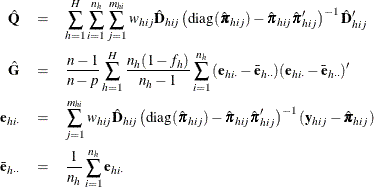
and  is the matrix of partial derivatives of the link function
  with respect to
  and
and  and the response probabilities
  are evaluated at .
If you specify the TECHNIQUE=NEWTON
option in the MODEL statement to request the Newton-Raphson algorithm
, the matrix  is replaced by the negative (expected) Hessian matrix when the estimated covariance matrix
  is computed.
Adjustments to the Variance Estimation
The factor  in the computation of the matrix
  reduces the small sample bias associated with using the estimated function to calculate deviations (Morel 1989; Hidiroglou, Fuller, and Hickman 1980). For simple random sampling, this factor contributes to the degrees-of-freedom correction applied to the residual mean square
for ordinary least squares in which p parameters are estimated. By default, the procedure uses this adjustment in Taylor series variance estimation. It is equivalent
to specifying the VADJUST=DF
option in the MODEL statement. If you do not want to use this multiplier in the variance estimation, you can specify the
VADJUST=NONE
option in the MODEL statement to suppress this factor.
reduces the small sample bias associated with using the estimated function to calculate deviations (Morel 1989; Hidiroglou, Fuller, and Hickman 1980). For simple random sampling, this factor contributes to the degrees-of-freedom correction applied to the residual mean square
for ordinary least squares in which p parameters are estimated. By default, the procedure uses this adjustment in Taylor series variance estimation. It is equivalent
to specifying the VADJUST=DF
option in the MODEL statement. If you do not want to use this multiplier in the variance estimation, you can specify the
VADJUST=NONE
option in the MODEL statement to suppress this factor.
In addition, you can specify the VADJUST=MOREL
option to request an adjustment to the variance estimator for the model parameters , introduced by Morel (1989):
![\[ \hat V(\hat{\btheta })= \hat{\mb{Q}}^{-1} \hat{\mb{G}} \hat{\mb{Q}}^{-1} + \kappa \lambda \hat{\mb{Q}}^{-1} \]](images/statug_surveylogistic0218.png)
where for given nonnegative constants  and
and  ,
,
The adjustment  does the following:
-
reduces the small sample bias reflected in inflated Type I error rates
-
guarantees a positive-definite estimated covariance matrix provided that
 exists
-
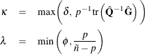
is close to zero when the sample size becomes large
In this adjustment,  is an estimate of the design effect, which has been bounded below by the positive constant . You can use DEFFBOUND= in the VADJUST=MOREL
option in the MODEL statement to specify this lower bound; by default, the procedure uses
is an estimate of the design effect, which has been bounded below by the positive constant . You can use DEFFBOUND= in the VADJUST=MOREL
option in the MODEL statement to specify this lower bound; by default, the procedure uses  . The factor
  converges to zero when the sample size becomes large, and has an upper bound . You can use ADJBOUND= in the VADJUST=MOREL
option in the MODEL statement to specify this upper bound; by default, the procedure uses
converges to zero when the sample size becomes large, and has an upper bound . You can use ADJBOUND= in the VADJUST=MOREL
option in the MODEL statement to specify this upper bound; by default, the procedure uses  .
.
Balanced Repeated Replication (BRR) Method
The balanced repeated replication (BRR) method requires that the full sample be drawn by using a stratified sample design
with two primary sampling units (PSUs) per stratum. Let H be the total number of strata. The total number of replicates R is the smallest multiple of 4 that is greater than H. However, if you prefer a larger number of replicates, you can specify the REPS=number
option. If a number  number Hadamard matrix
cannot be constructed, the number of replicates is increased until a Hadamard matrix becomes available.
number Hadamard matrix
cannot be constructed, the number of replicates is increased until a Hadamard matrix becomes available.
Each replicate is obtained by deleting one PSU per stratum according to the corresponding Hadamard matrix and adjusting the original weights for the remaining PSUs. The new weights are called replicate weights.
Replicates are constructed by using the first H columns of the  Hadamard matrix
. The rth (
Hadamard matrix
. The rth ( ) replicate is drawn from the full sample according to the rth row of the Hadamard matrix as follows:
-
If the
 element of the Hadamard matrix is 1, then the first PSU of stratum h is included in the rth replicate and the second PSU of stratum h is excluded.
-
If the
element of the Hadamard matrix is –1, then the second PSU of stratum h is included in the rth replicate and the first PSU of stratum h is excluded.
Note that the "first" and "second" PSUs are determined by data order in the input data set. Thus, if you reorder the data set and perform the same analysis by using BRR method, you might get slightly different results, because the contents in each replicate sample might change.
The replicate weights of the remaining PSUs in each half-sample are then doubled to their original weights. For more details about the BRR method, see Wolter (2007) and Lohr (2010).
By default, an appropriate Hadamard matrix is generated automatically to create the replicates. You can request that the Hadamard matrix be displayed by specifying the VARMETHOD=BRR(PRINTH) method-option. If you provide a Hadamard matrix by specifying the VARMETHOD=BRR(HADAMARD=) method-option, then the replicates are generated according to the provided Hadamard matrix.
You can use the VARMETHOD=BRR(OUTWEIGHTS=) method-option to save the replicate weights into a SAS data set.
Let be the estimated regression coefficients from the full sample for , and let  be the estimated regression coefficient from the rth replicate by using replicate weights. PROC SURVEYLOGISTIC estimates the covariance matrix of by
![\[ \hat{\mb{V}}(\hat{\btheta }) = \frac{1}{R} \sum _{r=1}^ R \left( {\hat{\btheta }_ r} - \hat{\btheta } \right) \left( {\hat{\btheta }_ r} - \hat{\btheta } \right)’ \]](images/statug_surveylogistic0229.png)
with H degrees of freedom, where H is the number of strata.
Fay’s BRR Method
Fay’s method is a modification of the BRR method, and it requires a stratified sample design with two primary sampling units (PSUs) per stratum. The total number of replicates R is the smallest multiple of 4 that is greater than the total number of strata H. However, if you prefer a larger number of replicates, you can specify the REPS= method-option.
For each replicate, Fay’s method uses a Fay coefficient  to impose a perturbation of the original weights in the full sample that is gentler than using only half-samples, as in the
traditional BRR method. The Fay coefficient can be set by specifying the FAY =
to impose a perturbation of the original weights in the full sample that is gentler than using only half-samples, as in the
traditional BRR method. The Fay coefficient can be set by specifying the FAY =  method-option. By default,
  if the FAY
method-option is specified without providing a value for (Judkins 1990; Rao and Shao 1999). When
if the FAY
method-option is specified without providing a value for (Judkins 1990; Rao and Shao 1999). When  , Fay’s method becomes the traditional BRR
method. For more details, see Dippo, Fay, and Morganstein (1984); Fay (1984, 1989); Judkins (1990).
, Fay’s method becomes the traditional BRR
method. For more details, see Dippo, Fay, and Morganstein (1984); Fay (1984, 1989); Judkins (1990).
Let H be the number of strata. Replicates are constructed by using the first H columns of the Hadamard matrix
, where R is the number of replicates,  . The rth () replicate is created from the full sample according to the rth row of the Hadamard matrix as follows:
-
If the
element of the Hadamard matrix is 1, then the full sample weight of the first PSU in stratum h is multiplied by and the full sample weight of the second PSU is multiplied by  to obtain the rth replicate weights.
-
If the
element of the Hadamard matrix is –1, then the full sample weight of the first PSU in stratum h is multiplied by and the full sample weight of the second PSU is multiplied by to obtain the rth replicate weights.
You can use the VARMETHOD=BRR(OUTWEIGHTS=) method-option to save the replicate weights into a SAS data set.
By default, an appropriate Hadamard matrix is generated automatically to create the replicates. You can request that the Hadamard matrix be displayed by specifying the VARMETHOD=BRR(PRINTH) method-option. If you provide a Hadamard matrix by specifying the VARMETHOD=BRR(HADAMARD=) method-option, then the replicates are generated according to the provided Hadamard matrix.
Let be the estimated regression coefficients from the full sample for . Let be the estimated regression coefficient obtained from the rth replicate by using replicate weights. PROC SURVEYLOGISTIC estimates the covariance matrix of by
![\[ \hat{\mb{V}}(\hat{\btheta }) = \frac{1}{R(1-{\epsilon })^2} \sum _{r=1}^ R \left( {\hat{\btheta }_ r} - \hat{\btheta } \right) \left( {\hat{\btheta }_ r} - \hat{\btheta } \right)’ \]](images/statug_surveylogistic0236.png)
with H degrees of freedom, where H is the number of strata.
Jackknife Method
The jackknife method of variance estimation deletes one PSU at a time from the full sample to create replicates. The total
number of replicates R is the same as the total number of PSUs. In each replicate, the sample weights of the remaining PSUs are modified by the
jackknife coefficient  . The modified weights are called replicate weights.
The jackknife coefficient and replicate weights are described as follows.
Without Stratification
If there is no stratification in the sample design (no STRATA
statement), the jackknife coefficients are the same for all replicates:
![\[ \alpha _ r=\frac{R-1}{R} \, \, \, \, \, \mbox{where } r=1, 2, ..., R \]](images/statug_surveylogistic0238.png)
Denote the original weight in the full sample for the jth member of the ith PSU as  . If the ith PSU is included in the rth replicate (), then the corresponding replicate weight for the jth member of the ith PSU is defined as
![\[ w^{(r)}_{ij}={w_{ij}}/{\alpha _ r} \]](images/statug_surveylogistic0240.png)
With Stratification
If the sample design involves stratification, each stratum must have at least two PSUs to use the jackknife method.
Let stratum  be the stratum from which a PSU is deleted for the rth replicate. Stratum is called the donor stratum. Let
  be the total number of PSUs in the donor stratum
  . The jackknife coefficients are defined as
![\[ \alpha _ r=\frac{n_{{{\tilde h}_ r}}-1}{n_{{\tilde h}_ r}} \, \, \, \, \, \mbox{where } r=1, 2, ..., R \]](images/statug_surveylogistic0244.png)
Denote the original weight in the full sample for the jth member of the ith PSU as . If the ith PSU is included in the rth replicate (), then the corresponding replicate weight for the jth member of the ith PSU is defined as
![\[ w^{(r)}_{ij}=\left\{ \begin{array}{ll} w_{ij} & \mbox{if }\mi{i}\mbox{th PSU is not in the donor stratum }\tilde h_ r \\ w_{ij}/\alpha _ r & \mbox{if }\mi{i}\mbox{th PSU is in the donor stratum }\tilde h_ r \end{array} \right. \]](images/statug_surveylogistic0245.png)
You can use the VARMETHOD=JACKKNIFE(OUTJKCOEFS=) method-option to save the jackknife coefficients into a SAS data set and use the VARMETHOD=JACKKNIFE(OUTWEIGHTS=) method-option to save the replicate weights into a SAS data set.
If you provide your own replicate weights with a REPWEIGHTS
statement, then you can also provide corresponding jackknife coefficients with the JKCOEFS=
option. If you provide replicate weights but do not provide jackknife coefficients, PROC SURVEYLOGISTIC uses  as the jackknife coefficient for all replicates.
Let be the estimated regression coefficients from the full sample for . Let be the estimated regression coefficient obtained from the rth replicate by using replicate weights. PROC SURVEYLOGISTIC estimates the covariance matrix of by
![\[ \hat{\mb{V}}(\hat{\btheta }) = \sum _{r=1}^ R \alpha _ r \left( {\hat{\btheta }_ r} - \hat{\btheta } \right) \left( {\hat{\btheta }_ r} - \hat{\btheta } \right)’ \]](images/statug_surveylogistic0247.png)
with  degrees of freedom, where R is the number of replicates and H is the number of strata, or
  when there is no stratification.
Hadamard Matrix
A Hadamard matrix  is a square matrix whose elements are either 1 or –1 such that
![\[ \mb{H}\mb{H}’=k\mb{I} \]](images/statug_surveylogistic0250.png)
where k is the dimension of and  is the identity matrix of order k. The order k is necessarily 1, 2, or a positive integer that is a multiple of 4.
For example, the following matrix is a Hadamard matrix of dimension k = 8:
![\[ \begin{array}{rrrrrrrr} 1 & 1 & 1 & 1 & 1 & 1 & 1 & 1\\ 1 & -1 & 1 & -1 & 1 & -1 & 1 & -1\\ 1 & 1 & -1 & -1 & 1 & 1 & -1 & -1\\ 1 & -1 & -1 & 1 & 1 & -1 & -1 & 1\\ 1 & 1 & 1 & 1 & -1 & -1 & -1 & -1\\ 1 & -1 & 1 & -1 & -1 & 1 & -1 & 1\\ 1 & 1 & -1 & -1 & -1 & -1 & 1 & 1\\ 1 & -1 & -1 & 1 & -1 & 1 & 1 & -1 \end{array} \]](images/statug_surveylogistic0252.png)