The SPP Procedure
-
Overview

- Getting Started
-
Syntax
-
DetailsTesting for Complete Spatial RandomnessExploring Interpoint InteractionDistance Functions for Multitype Point PatternsBorder Edge Correction for Distance FunctionsConfidence Intervals for Summary StatisticsRipley-Rasson Window EstimatorCovariate Dependence TestsNonparametric Intensity EstimationInhomogeneous Poisson Process Model FittingNegative Binomial ModelingOutput Data SetsDisplayed OutputODS Table NamesODS Graphics
-
Examples
- References
Nonparametric Intensity Estimation
The KERNEL option in the PROCESS statement enables you to perform nonparametric intensity estimation. You can use five different
kernel types: Epanechnikov, Gaussian, uniform, triangular, and quartic (Silverman 1986), whose kernel functions are as follows, where 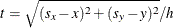 ,
,  ,
,  are the grid point coordinates, x and y are the point coordinates, and h is the bandwidth parameter:
-
Epanechnikov
![\[ K(t) = \begin{cases} \frac{3}{4}(1-\frac{t^{2}}{5})\frac{1}{\sqrt {5}}& |t|<\sqrt {5}\\ 0& \text {otherwise} \end{cases} \]](images/statug_spp0152.png)
-
Gaussian
![\[ K(t) = \frac{e^{-\frac{t^{2}}{2}}}{\sqrt {2\pi }} \]](images/statug_spp0153.png)
-
uniform
![\[ K(t) = \begin{cases} \frac{1}{2} & |t| < 1\\ 0 & \text {otherwise} \end{cases} \]](images/statug_spp0154.png)
-
triangular
![\[ K(t) = \begin{cases} 1-|t| & |t| < 1\\ 0 & \text {otherwise} \end{cases} \]](images/statug_spp0155.png)
-
quartic
![\[ K(t) = \begin{cases} \frac{15}{16}(1-t^{2})^{2} & |t| < 1\\ 0& \text {otherwise} \end{cases} \]](images/statug_spp0156.png)
Given the preceding kernel definitions, the nonparametric intensity estimate can be computed as
![\[ \lambda (s) = \sum _{i=1}^{n} h^{-2} \times K\left(\frac{s-s_ i}{h}\right) \]](images/statug_spp0157.png)
where h is the fixed bandwidth. In practice, nonparametric intensity estimation also involves an edge correction. By default, PROC
SPP divides the nonparametric estimate  by an edge correction factor
![\[ \rho (s) = \int _ A h^{-2} \times K\left(\frac{s-s_ i}{h}\right) \]](images/statug_spp0158.png)
where A is the study area. The choice of the bandwidth parameter that nonparametric intensity estimation requires is more important than the choice of the kernel type itself (Silverman 1986). The bandwidth can be spatially fixed or spatial varying. If the bandwidth is spatially varying, it is called adaptive kernel estimation. For adaptive kernel estimation, the SPP procedure uses the technique suggested in Silverman (1986, p. 101) and Diggle, Rowlingson, and Su (2005, p. 426), which is computed in two steps:
-
Use an initial bandwidth h to compute pilot estimates of the first-order intensity as
![\[ \lambda _0(s) = \sum _{i=1}^{n} h^{-2} \times K\left(\frac{s-s_ i}{h}\right) \]](images/statug_spp0159.png)
where K(.) is a kernel.
-
Compute bandwidth factors as
![\[ h_ i = h \times \left( \frac{\lambda _0(s)}{\widehat{g}} \right)^{-0.5} \]](images/statug_spp0160.png)
where
 is the geometric mean of the pilot estimates
  .
.
Based on the computed bandwidth estimates,  , the nonparametric intensity estimates are computed as
![\[ \lambda (s) = \sum _{i=1}^{n} h_ i^{-2} \times K\left(\frac{s-s_ i}{h_ i}\right) \]](images/statug_spp0164.png)
In PROC SPP, adaptive kernel estimation does not incorporate edge correction.