The CALIS Procedure

Example 26.32 Longitudinal Factor Analysis

The following example (McDonald; 1980) illustrates both the ability of PROC CALIS to formulate complex covariance structure analysis problems by the generalized COSAN matrix model and the use of programming statements to impose nonlinear constraints on the parameters. The example is a longitudinal factor analysis that uses the Swaminathan (1974) model. For tests, occasions, and factors, the covariance structure model is formulated as follows:

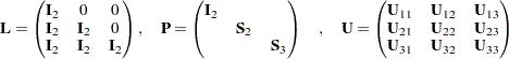
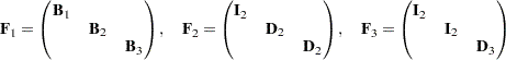
The Swaminathan longitudinal factor model assumes that the factor scores for each () common factor change from occasion to occasion () according to a first-order autoregressive scheme. The matrix contains the factor loading matrices , , and (each is ). The matrices and 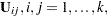are diagonal, and the matrices and are subjected to the constraint

Although the covariance structure model looks pretty complicated, it poses no problem for the COSAN model specifications. Since the constructed correlation matrix given by McDonald (1980) is singular, only unweighted least squares (METHOD=LS) estimates can be computed. The following statements specify the COSAN model for the correlation structures.

data Mcdon(TYPE=CORR);
Title "Swaminathan's Longitudinal Factor Model, Data: McDONALD(1980)";     
Title2 "Constructed Singular Correlation Matrix, GLS & ML not possible";   
   _TYPE_ = 'CORR'; INPUT _NAME_ $ obs1-obs9;                              
   datalines;                                                              
obs1  1.000    .      .      .      .      .      .      .      .          
obs2   .100  1.000    .      .      .      .      .      .      .          
obs3   .250   .400  1.000    .      .      .      .      .      .          
obs4   .720   .108   .270  1.000    .      .      .      .      .          
obs5   .135   .740   .380   .180  1.000    .      .      .      .          
obs6   .270   .318   .800   .360   .530  1.000    .      .      .          
obs7   .650   .054   .135   .730   .090   .180  1.000    .      .          
obs8   .108   .690   .196   .144   .700   .269   .200  1.000    .          
obs9   .189   .202   .710   .252   .336   .760   .350   .580  1.000        
     ;

proc calis data=Mcdon method=ls nobs=100 corr;
cosan 
   var = obs1-obs9, 
   F1(6,GEN) * F2(6,DIA) * F3(6,DIA) * L(6,LOW) * F3(6,DIA,INV)
             * F2(6,DIA,INV) * P(6,DIA) + U(9,SYM);                      
   matrix F1 
            [1 , @1] = x1-x3,                                                  
            [2 , @2] = x4-x5,                                               
            [4 , @3] = x6-x8,                                           
            [5 , @4] = x9-x10,                                          
            [7 , @5] = x11-x13,                                         
            [8 , @6] = x14-x15;                                         
   matrix F2                                                                 
            [1,1]= 2 * 1. x16 x17 x16 x17;                                 
   matrix F3                                                                 
            [1,1]= 4 * 1. x18 x19;                                         
   matrix L                                                                  
            [1,1]= 6 * 1.,                                                 
            [3,1]= 4 * 1.,                                                 
            [5,1]= 2 * 1.;                                                 
   matrix P                                                                  
            [1,1]= 2 * 1. x20-x23;                                         
   matrix U                                                                  
            [1,1]= x24-x32,                                                
            [4,1]= x33-x38,                                                
            [7,1]= x39-x41;                                                
   bounds 0. <= x24-x32,                                                     
         -1. <= x16-x19 <= 1.;   
   /* SAS programming statements for dependent parameters */                                            
   x20 = 1. - x16 * x16;                                                     
   x21 = 1. - x17 * x17;                                                     
   x22 = 1. - x18 * x18;                                                     
   x23 = 1. - x19 * x19;                                                     
run;                 

In the PROC CALIS statement, you use the NOBS= option to specify the number of observations. The CORR option requests the analysis of the correlation matrix.

In the COSAN statement, you list the observed variables for the analysis in the VAR= option. Then you specify the formula for the covariance structures. Notice that in the covariance structure formula, some matrices are specified twice. That is, matrix and appear in two different places. Matrices with the same name means that they are identical—which certainly makes sense. In addition, you can apply different transformations to the same matrix in different locations of the matrix formula. For example, you do not transform matrix in the first location, but the same matrix is inverted (INV) later in the expression. Similarly for matrix .

Next, you define the parameters in the six distinct model matrices by six MATRIX statements. Each matrix has some specific patterns under the covariance structure model. For the matrix, it has the following pattern for the free parameters in the model:

            col1  col2  col3  col4  col5  col6 
     row1    x       
     row2    x     x 
     row3    x     x 
     row4                x        
     row5                x     x       
     row6                x     x    
     row7                            x       
     row8                            x     x 
     row9                            x     x 

To specify these parameters, you can use some shorthand notation in the MATRIX statement. For example, in the first entry of the MATRIX statement for matrix , you use the notation [1,@1]. This means that the parameter specification starts with the [1,1] element and proceeds to the next element while fixing the column number at 1. Hence, parameters x1–x3 are specified for the , , and elements, respectively. Similarly, you specify other parameters in the matrix in a column by column fashion.

If you do not use the @ sign in the specification, the parameters are assigned differently. For example, in the specification of the matrix, the first entry in the corresponding MATRIX statement also starts with the [1,1] element. But it proceeds down to [2,2], [3,3], and so on because the @ sign is not used to fix any column or row number. As a result, the MATRIX statement for specifies the following pattern:

            col1  col2  col3  col4  col5  col6 
     row1    1       
     row2          1 
     row3    1           1
     row4          1           1        
     row5    1           1           1       
     row6          1           1           1    

The unspecified elements are fixed zeros in the model.

Similarly, you specify the diagonal matrices , , and , and the symmetric matrix .

You also set bounds for some parameters in the BOUNDS statement and some dependent parameters in the SAS programming statements.

Output 26.32.1 shows the correlation structures and the model matrices in the analysis. All appear to be intended.

PROC CALIS finds a converged solution for the estimation problem. Output 26.32.2, Output 26.32.3, and Output 26.32.4 show the estimation results of the , , and matrices, respectively.

Output 26.32.2 Estimation of the Matrix of the Longitudinal Factor Model

Model Matrix F1
(9 x 6 General Rectangular Matrix)
	Col1	Col2	Col3	Col4	Col5	Col6
obs1	0.3515 [x1]	0	0	0	0	0
obs2	0.2871 [x2]	0.9528 [x4]	0	0	0	0
obs3	0.7101 [x3]	0.2059 [x5]	0	0	0	0
obs4	0	0	0.4204 [x6]	0	0	0
obs5	0	0	0.4303 [x7]	0.9027 [x9]	0	0
obs6	0	0	0.8591 [x8]	0.1772 [x10]	0	0
obs7	0	0	0	0	0.3487 [x11]	0
obs8	0	0	0	0	0.5924 [x12]	-0.1971 [x14]
obs9	0	0	0	0	0.9987 [x13]	0.0871 [x15]

Output 26.32.3 Estimation of the Matrix of the Longitudinal Factor Model

Model Matrix F2
(6 x 6 Diagonal Matrix)
	Col1	Col2	Col3	Col4	Col5	Col6
Row1	1.0000	0	0	0	0	0
Row2	0	1.0000	0	0	0	0
Row3	0	0	0.8939 [x16]	0	0	0
Row4	0	0	0	0.5806 [x17]	0	0
Row5	0	0	0	0	0.8939 [x16]	0
Row6	0	0	0	0	0	0.5806 [x17]

Output 26.32.4 Estimation of the Matrix of the Longitudinal Factor Model

Model Matrix F3
(6 x 6 Diagonal Matrix)
	Col1	Col2	Col3	Col4	Col5	Col6
Row1	1.0000	0	0	0	0	0
Row2	0	1.0000	0	0	0	0
Row3	0	0	1.0000	0	0	0
Row4	0	0	0	1.0000	0	0
Row5	0	0	0	0	0.5963 [x18]	0
Row6	0	0	0	0	0	1.0000 [x19]

Output 26.32.5 shows the estimation results of the matrix, which is a fixed matrix that contains only 0 or 1 for its elements.

Output 26.32.5 Estimation of the Matrix of the Longitudinal Factor Model

Model Matrix L
(6 x 6 Lower Triangular Matrix)
	Col1	Col2	Col3	Col4	Col5	Col6
Row1	1.0000	0	0	0	0	0
Row2	0	1.0000	0	0	0	0
Row3	1.0000	0	1.0000	0	0	0
Row4	0	1.0000	0	1.0000	0	0
Row5	1.0000	0	1.0000	0	1.0000	0
Row6	0	1.0000	0	1.0000	0	1.0000

Output 26.32.6 shows the estimation results of the matrix. Notice that parameter estimate x23 falls on the lower boundary at zero.

Output 26.32.6 Estimation of the Matrix of the Longitudinal Factor Model

Model Matrix P
(6 x 6 Diagonal Matrix)
	Col1	Col2	Col3	Col4	Col5	Col6
Row1	1.0000	0	0	0	0	0
Row2	0	1.0000	0	0	0	0
Row3	0	0	0.2010 [x20]	0	0	0
Row4	0	0	0	0.6629 [x21]	0	0
Row5	0	0	0	0	0.6444 [x22]	0
Row6	0	0	0	0	0	0 [x23]

In fact, PROC CALIS routinely checks for zero values for the estimates on the diagonal of the central symmetric matrices. In this case, you get the following messages regarding the estimation of matrix :

WARNING: Although all predicted variances for the observed variables are  
         positive, the corresponding predicted covariance matrix is not 
         positive definite. It has one negative eigenvalue.
WARNING: The estimated variance of variable 6 is essentially zero in the 
         central matrix P of term 1 of the COSAN model.
WARNING: The central matrix P of term 1 of the COSAN model is not positive 
         definite. It has one zero eigenvalue.

Output 26.32.7 shows the estimation results of the matrix. Parameter estimates x28 and x32 fall on the lower boundary at zero. PROC CALIS issues the following messages regarding the estimation of matrix :

WARNING: The estimated variance of obs5 is essentially zero in the central 
         matrix U of term 2 of the COSAN model.
WARNING: The estimated variance of obs9 is essentially zero in the central
         matrix U of term 2 of the COSAN model.
WARNING: The central matrix U of term 2 of the COSAN model is not positive
         definite. It has 3 negative eigenvalues.

Output 26.32.7 Estimation of the Matrix of the Longitudinal Factor Model

Model Matrix U
(9 x 9 Symmetric Matrix)
	obs1	obs2	obs3	obs4	obs5	obs6	obs7	obs8	obs9
obs1	0.8764 [x24]	0	0	0.5879 [x33]	0	0	0.5847 [x39]	0	0
obs2	0	0.009683 [x25]	0	0	0.1302 [x34]	0	0	0.7084 [x40]	0
obs3	0	0	0.4533 [x26]	0	0	0.2335 [x35]	0	0	0.3215 [x41]
obs4	0.5879 [x33]	0	0	0.8233 [x27]	0	0	0.6426 [x36]	0	0
obs5	0	0.1302 [x34]	0	0	0 [x28]	0	0	0.7259 [x37]	0
obs6	0	0	0.2335 [x35]	0	0	0.2305 [x29]	0	0	0.2329 [x38]
obs7	0.5847 [x39]	0	0	0.6426 [x36]	0	0	0.8784 [x30]	0	0
obs8	0	0.7084 [x40]	0	0	0.7259 [x37]	0	0	0.6102 [x31]	0
obs9	0	0	0.3215 [x41]	0	0	0.2329 [x38]	0	0	0 [x32]

Because this formulation of Swaminathan’s model in general leads to an unidentified problem, the results given here are different from those reported by McDonald (1980). The displayed output of PROC CALIS also indicates that the fitted central model matrices and are not positive-definite. The BOUNDS statement constrains the diagonals of the matrices and to be nonnegative, but this cannot prevent from having three negative eigenvalues. The fact that many of the published results for more complex models in covariance structure analysis are connected to unidentified problems implies that more theoretical work should be done to study the general features of such models.