IMSTAT Procedure (Analytics)
- Syntax
 Procedure SyntaxPROC IMSTAT (Analytics) StatementAGGREGATE StatementARM StatementASSESS StatementBOXPLOT StatementCLUSTER StatementCORR StatementCROSSTAB StatementDECISIONTREE StatementDISTINCT StatementFORECAST StatementFREQUENCY StatementGENMODEL StatementGLM StatementGROUPBY StatementHISTOGRAM StatementHYPERGROUP StatementKDE StatementLOGISTIC StatementMDSUMMARY StatementNEURAL StatementOPTIMIZE StatementPERCENTILE StatementRANDOMWOODS StatementREGCORR StatementSUMMARY StatementTEXTPARSE StatementTOPK StatementTRANSFORM StatementQUIT Statement
 - Overview
- Using
- Examples Calculating Percentiles and QuartilesRetrieving Box ValuesRetrieving Box Plot Values with the NOUTLIERLIMIT= OptionRetrieving Distinct Value Counts and GroupingPerforming a Cluster AnalysisPerforming a Pairwise CorrelationCrosstabulation with Measures of Association and Chi-Square TestsTraining and Validating a Decision TreeStoring and Scoring a Decision TreePerforming a Multi-Dimensional SummaryFitting a Regression ModelForecasting and Automatic ModelingForecasting with Goal SeekingAggregating Time Series DataTraining and Validating a Neural NetworkPredicting Email Spam and Assessing the ModelTransforming Variables with Imputation and Binning
OPTIMIZE Statement
The OPTIMIZE statement performs a non-linear optimization of an objective function that is defined through a SAS program. The expression defined in the SAS program and its analytic first and second derivatives are compiled into executable code. The code is then executed in multiple threads against the data in an in-memory table. Like all other IMSTAT statements, the calculations are performed by the server. You can choose from several first-order and second-order optimization algorithms.
Syntax
OPTIMIZE Statement Options
ALPHA=number
specifies a number between 0 and 1 from which to determine the confidence level for approximate confidence intervals of the parameter estimates. The default is α = 0.05, which leads to 100 x (1- α)% = 95% confidence limits for the parameter estimates.
| Default | 0.05 |
BOUNDS=(boundary-specification<, boundary-specification,...>)
specifies boundary values for the parameters. A boundary-specification is specified in the following form:
parameter-name
specifies the parameter
operator
is one of >=, GE, <=, LE, >, GT, <, LT, =, EQ.
value
specifies the boundary value
| Alias | BOUND= |
| Example | BOUNDS=(s2 > 0, beta2 >= 0.2) |
CODE=file-reference
specifies a file reference
to the SAS program that defines the objective function. The program
must make an assignment to the reserved symbol _OBJFNC_.
The server then minimizes the negative of that function (or maximize
the function). In other words, you should specify _OBJFNC_ to
be the function that you want to maximize across the in-memory table.
The actual optimization is carried out as a minimization problem.
| Alias | PGM= |
DEFSTART=value
specifies the default starting value for parameters whose starting value has not been specified. The default value, 1, might not work well depending on the optimization.
| Alias | DEFVAL= |
| Default | 1 |
DUD
specifies that you do not want to use analytic derivatives in the optimization. The option name is an acronym for "do not use derivatives." Instead, the server calculates gradient vectors and Hessian matrices from finite difference approximations. Generally, you should not rely on derivatives calculated from finite differences if analytic derivatives are available. However, this option is useful in situations where the objective function is not calculated independently for each row of data. If derivatives of the objective function depend on lagged values, which are themselves functions of the parameters, then finite difference derivatives are called for.
| Alias | NODERIVATIVES |
FCONV=r
specifies a relative function convergence criterion. For all techniques except NMSIMP, termination requires a small relative change of the function value in successive iterations. Suppose that Ψ is the p × 1 vector of parameter estimates in the optimization, and the objective function at the kth iteration is denoted as f(Ψ)k. Then, the FCONV criterion is met if
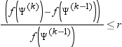
| Default | r=10-FDIGITS where FDIGITS is -log10(e) and e is the machine precision. |
GCONV=r
specifies a relative gradient convergence criterion. For all optimization techniques except CONGRA and NMSIMP, termination requires that the normalized predicted function reduction is small. The default value is r = 1e-8. Suppose that Ψ is the p × 1 vector of parameter estimates in the optimization with ith element Ψi. The objective function, its p × 1 gradient vector, and its p × p Hessian matrix are denoted, f(Ψ), g(Ψ), and H(Ψ ), respectively. Then, if superscripts denote the iteration count, the normalized predicted function reduction at iteration k is

ITDETAIL
requests that the server produce an iteration history table for the optimization. This table displays the objective function, its absolute change, and the largest absolute gradient across the iterations.
MAXFUNC=n
specifies the maximum number n of function calls in the iterative model fitting process. The default value depends on the optimization technique as follows:
|
Optimization Technique
|
Default Number of Function
Calls
|
|---|---|
|
TRUREG, NRRIDG, and
NEWRAP
|
125
|
|
QUANEW and DBLDOG
|
500
|
|
CONGRA
|
1000
|
|
NMSIMP
|
3000
|
| Alias | MAXFU= |
MAXITER=i
specifies the maximum number of iterations in the iterative model fitting process. The default value depends on the optimization technique as follows:
|
Optimization Technique
|
Default Number of Iterations
|
|---|---|
|
TRUREG, NRRIDG, and
NEWRAP
|
50
|
|
QUANEW and DBLDOG
|
200
|
|
CONGRA
|
400
|
|
NMSIMP
|
1000
|
| Alias | MAXIT= |
MAXTIME=t
specifies an upper limit of t seconds of CPU time for the optimization process. The default value is the largest floating-point double representation value for the hardware used by the SAS LASR Analytic Server. Note that the time specified by the MAXTIME= option is checked only once at the end of each iteration. The time is measured on the root node for the server. Therefore, the actual running time can be longer than the value specified by the MAXTIME= option.
MINITER=i
specifies the minimum number of iterations.
| Alias | MINIT= |
| Default | 0 |
NBEST=k
requests that only the k best points in the starting value grid are reproduced in the "Starting Values" table. By default, the objective function is initially evaluated at all points in the starting value grid and the "Starting Values" table contains one row for each point on the grid. If you specify the NBEST= option, then only the k points with the smallest objective function value are shown.
| Alias | BEST= |
NOEMPTY
requests that result sets for optimizations without usable data are not generated.
NOPREPARSE
specifies to prevent pre-parsing and pre-generating the program code that is referenced in the CODE= option. If you know the code is correct, you can specify this option to save resources. The code is always parsed by the server, but you might get more detailed error messages when the procedure parses the code rather than the server. The server assumes that the code is correct. If the code fails to compile, the server indicates that it could not parse the code, but not where the error occurred.
| Alias | NOPREP |
NOSTDERR
specifies to prevent calculating standard errors of the parameter estimates. The calculation of standard errors requires the derivation of the Hessian or cross-product Jacobian. If you do not want standard errors, p-values, or confidence intervals for the parameter estimates, then specifying this option saves computing resources.
| Alias | NOSTD |
PARAMETERS=(parameter-specification <, parameter-specification ...>)
specifies the parameters in the optimization and the starting values. You do not have to specify parameters and you do not have to specify starting values. If you omit the starting values, the default starting value is assigned. This default value is 1.0 and can be modified with the DEFSTART= option.
| Alias | PARMS= |
| Examples | DEFSTART=0; PARMS=(Intercept = 6, a_0, b_0, c_0, x_1, x_2, x_3); |
| PARMS=(beta1 = -3.22, beta2 = 0.5 0.47 0.6, beta3 = -2.45 -2.0, s2 = 0.5); |
RESTRICT=(one-restriction <, one-restriction>)
specifies linear equality and inequality constraints for the optimization. A single restriction takes on the general form
coefficient parameter ... coefficient parameter operator value
| Examples | RESTRICT=(1 beta1 -2 beta2 > 3) |
| RESTRICT=(1 dose1 -1 dose2 = 0, 1 logd1 -1 logd2 = 0) |
SAVE=table-name
saves the result table so that you can use it in other IMSTAT procedure statements like STORE, REPLAY, and FREE. The value for table-name must be unique within the scope of the procedure execution. The name of a table that has been freed with the FREE statement can be used again in subsequent SAVE= options.
SETSIZE
requests that the server estimate the size of the result set. The procedure does not create a result table if the SETSIZE option is specified. Instead, the procedure reports the number of rows that are returned by the request and the expected memory consumption for the result set (in KB). If you specify the SETSIZE option, the SAS log includes the number of observations and the estimated result set size. See the following log sample:
NOTE: The LASR Analytic Server action request for the STATEMENT
      statement would return 17 rows and approximately
3.641 kBytes of data.TECHNIQUE=
specifies the optimization technique.
| CONGRA (CG) | performs a conjugate-gradient optimization. |
| DBLDOG (DD) | performs a version of the double-dogleg optimization. |
| DUQUANEW (DQN) | performs a (dual) quasi-Newton optimization. |
| NMSIMP (NS) | performs a Nelder-Mead simplex optimization. |
| NONE | specifies not to perform any optimization. This value can be used to perform a grid search without optimization. |
| NEWRAP (NRA) | performs a (modified) Newton-Raphson optimization that combines a line-search algorithm with ridging. |
| NRRIDG (NRR) | performs a (modified) Newton-Raphson optimization with ridging. |
| QUANEW (QN) | performs a quasi-Newton optimization. |
| TRUREG (TR) | performs a trust-region optimization. |
| Alias | TECH= |
| Default | DUQUANEW |
Details
ODS Table Names
|
ODS Table Name
|
Description
|
Option
|
|---|---|---|
|
OptParameters
|
Starting values for
optimization
|
Default
|
|
OptIterHistory
|
Iteration history
|
ITDETAILS
|
|
ConvergenceStatus
|
Convergence status
|
Default
|
|
OptFitStatistics
|
Fit statistics
|
Default
|
|
OptParameterEstimates
|
Parameter estimates
for optimization
|
Default
|