IMSTAT Procedure (Analytics)
- Syntax
 Procedure SyntaxPROC IMSTAT (Analytics) StatementAGGREGATE StatementARM StatementASSESS StatementBOXPLOT StatementCLUSTER StatementCORR StatementCROSSTAB StatementDECISIONTREE StatementDISTINCT StatementFORECAST StatementFREQUENCY StatementGENMODEL StatementGLM StatementGROUPBY StatementHISTOGRAM StatementHYPERGROUP StatementKDE StatementLOGISTIC StatementMDSUMMARY StatementNEURAL StatementOPTIMIZE StatementPERCENTILE StatementRANDOMWOODS StatementREGCORR StatementSUMMARY StatementTEXTPARSE StatementTOPK StatementTRANSFORM StatementQUIT Statement
 - Overview
- Using
- Examples Calculating Percentiles and QuartilesRetrieving Box ValuesRetrieving Box Plot Values with the NOUTLIERLIMIT= OptionRetrieving Distinct Value Counts and GroupingPerforming a Cluster AnalysisPerforming a Pairwise CorrelationCrosstabulation with Measures of Association and Chi-Square TestsTraining and Validating a Decision TreeStoring and Scoring a Decision TreePerforming a Multi-Dimensional SummaryFitting a Regression ModelForecasting and Automatic ModelingForecasting with Goal SeekingAggregating Time Series DataTraining and Validating a Neural NetworkPredicting Email Spam and Assessing the ModelTransforming Variables with Imputation and Binning
Example 12: Forecasting and Automatic Modeling
Details
This IMSTAT procedure
example demonstrates using the FORECAST statement in its simplest
use and when used with independent variables.
Program
libname example sasiola host="grid001.example.com" port=10010 tag='hps';

data example.pricedata;
    set sashelp.pricedata;
    where region=1 and product=1 and line=1;
run;

proc imstat data=example.pricedata;
    forecast date / vars =sale  1
                    lead =4
                    info;
run;

    forecast date / vars =sale
                    lead =4
                    info
                    indep=(price discount);  2

    ods output forecast out=work.forecast2;  3
quit;

proc sgplot data=work.forecast2;
    format date monyy7.; /* monyy5.; */
    band x=date lower=lower upper=upper /
       legendlabel="95% CLI" name="band";

    series x=date y=predict / lineattrs=GraphPrediction name="predict";
    series x=date y=actual / name="actual";

    keylegend "actual" "predict" "band" / location=inside
        position=bottomright;
run;
Program Description
-
The first FORECAST statement shows the simplest usage. The Sale variable is forecasted and the Date variable is used as the time stamp for identifying the time series. The LEAD=4 option specifies to forecast four intervals into the future.
-
The second FORECAST statement is similar to the first, but specifies independent variables in the data. In this case, the server performs time series model building and variable selection. Variables Price and Discount are candidates for the independent variables.
-
The ODS statement is used to save the results of the second forecast in a temporary SAS data set that is named Forecast2. You can use the data set with the SGPLOT procedure or other graphics procedures for plotting the forecast. For information about plots, see SGPLOT Procedure in SAS ODS Graphics: Procedures Guide.
Output
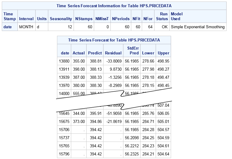
The following display
shows the results for the two FORECAST statements. The first display
shows the results for the forecast information and then the forecasted
time series of the Sale variable in the Pricedata data set.
The Date column contains
the value of the time stamp. Observed values of the time series are
identified by a nonmissing value for the variable named Actual variable.
For example, the mean value of Sale at Date=13880 is 355.00. The
Predict column contains the predicted value under the chosen model
and the Residual column is the difference between the observed value
in the Actual column and the predicted value.
The StdErrPred column
contains the standard error of the predicted value. This is a measure
of the precision of predicting the value of Sale for the particular
time stamp under the model used. The Lower and Upper columns are the
confidence limits for the prediction.
The observations with
missing values for column Actual at the end of the table contain the
forecasted value in column Predict. Notice how the value of the prediction
standard error grows quickly as the forecast extends beyond the observed
time stamps. The width of the confidence interval grows accordingly.
The further that you predict into the future, the less precise the
prediction is. The result table contains several columns not shown
in the following display. These columns identify the table, the analysis
variable, and the aggregator. You can materialize those columns by
writing the table to a SAS data set.
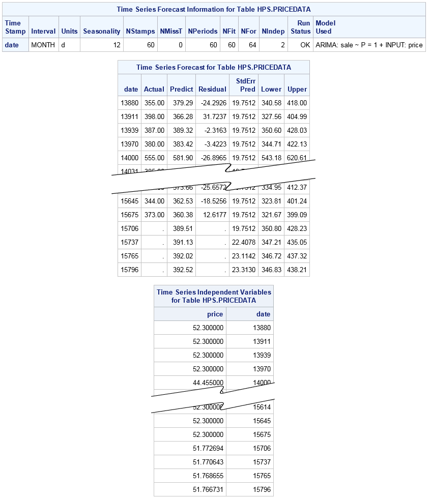
The second FORECAST
statement specifies independent variables in the data. In this case,
the server performs time series model building and variable selection
and then returns the best-fitting time series model and values for
the selected independent variables.
The forecast information
table indicates that an ARIMA model with variable Price as the independent
variable was chosen as the best-fitting model. Note that in automatic
modeling mode it is possible that none of the independent variables
specified in the INDEP= option are used in the final model. The model
then falls back to an exponential smoothing model as in previous FORECAST
statement.
In addition, when one
or more independent variables are selected for the model, the output
includes a table with the values for the independent variables. Notice
that the independent variables are also forecast into the lead horizon.
The last time stamp in the input data set for the dependent and independent
variables is Date=15675 with Price having an observed value of 52.3.
Copyright © SAS Institute Inc. All Rights Reserved.