The QUANTSELECT Procedure

Example 96.5 Quantile Process Regression
Quantile process regression fits quantile regression models for the entire range of quantile levels from 0 to 1, which can estimate the entire probability distribution of a response variable conditional on its covariates. This example demonstrates how you can conduct quantile process regression analysis by using the QUANTSELECT procedure.
Parameter Estimates for Quantile Process Regression
The following statements simulate the data set analysisData, solve a quantile process regression problem on the data set, and store the quantile process parameter estimates in the data
set quantProcessEst. The data set analysisData contains one response y and two covariates, x1 and x2. The distribution of y conditional on x1 and x2 gradually changes from a normal distribution to an exponential distribution.
%let seed=123;
%let n=6001;
%let model=x1 x2;
data analysisData;
   do i=1 to &n;
      x1=(i-1)/(&n-1);
      x2=(1-x1)*(1-x1);
      y =x1*ranexp(&seed)+x2*(rannor(&seed)-3);
      output;
   end;
run;
proc quantselect data=analysisData;
   ods output ProcessEst=quantProcessEst;
   model y = &model / quantile=process(ntau=all) selection=none;
run;

proc print data=quantProcessEst(obs=10);
run;
Output 96.5.1 shows the first 10 parameter estimates of the quantile process. For more information about parameter estimates for the quantile process, see the section Parameter Estimates for Quantile Process.
Output 96.5.1: Quantile Process Parameter Estimates
| Obs | QuantileLabel | QuantileLevel | Intercept | x1 | x2 |
|---|---|---|---|---|---|
| 1 | t0 | 0.000000 | -1.3799 | 1.3982 | -4.3156 |
| 2 | t1 | 0.000121 | -1.3799 | 1.3982 | -4.3156 |
| 3 | t2 | 0.000248 | -0.8210 | 0.8386 | -5.0420 |
| 4 | t3 | 0.000283 | 0.2030 | -0.2006 | -6.3677 |
| 5 | t4 | 0.000322 | 0.3065 | -0.3098 | -6.5001 |
| 6 | t5 | 0.000436 | 0.4713 | -0.4854 | -6.7102 |
| 7 | t6 | 0.000541 | 0.2788 | -0.2812 | -6.2666 |
| 8 | t7 | 0.000592 | 0.1957 | -0.1939 | -6.0724 |
| 9 | t8 | 0.000760 | 0.1940 | -0.1915 | -6.0704 |
| 10 | t9 | 0.000880 | 0.1987 | -0.1963 | -6.0765 |
To reduce the computation complexity, you can also approximate the quantile process regression by using the NTAU=n suboption of the QUANTILE=PROCESS option. The following statements approximate the quantile process by using NTAU=10:
proc quantselect data=analysisData;
   ods output ProcessEst=quantApproxProcessEst;
   model y = &model / quantile=process(ntau=10) selection=none;
run;

proc print data=quantApproxProcessEst;
run;
Output 96.5.2 shows the approximate quantile process parameter estimates. If you specify the NTAU=n option, the approximate quantile process is computed at n equally spaced quantile levels:  besides three control quantile levels
  .
.
Output 96.5.2: Approximate Quantile Process Parameter Estimates
| Obs | QuantileLabel | QuantileLevel | Intercept | x1 | x2 |
|---|---|---|---|---|---|
| 1 | t0 | 0.000000 | -1.3799 | 1.3982 | -4.3156 |
| 2 | t1 | 0.090909 | 0.6051 | -0.5449 | -4.8257 |
| 3 | t2 | 0.181818 | 0.5273 | -0.3595 | -4.3719 |
| 4 | t3 | 0.272727 | 0.3871 | -0.0764 | -3.9561 |
| 5 | t4 | 0.363636 | 0.3381 | 0.0980 | -3.6935 |
| 6 | t5 | 0.454545 | 0.1747 | 0.4300 | -3.2961 |
| 7 | t6 | 0.500000 | 0.0197 | 0.6928 | -3.0160 |
| 8 | t7 | 0.545455 | -0.1102 | 0.9365 | -2.7518 |
| 9 | t8 | 0.636364 | -0.3543 | 1.4418 | -2.2749 |
| 10 | t9 | 0.727273 | -0.6169 | 2.0165 | -1.7714 |
| 11 | t10 | 0.818182 | -1.0307 | 2.8540 | -1.0614 |
| 12 | t11 | 0.909091 | -1.4056 | 3.8941 | -0.3141 |
| 13 | t12 | 1.000000 | -1.9936 | 9.1022 | 1.2334 |
Observation Quantile Levels
Quantile process regression can estimate observation quantile levels for any valid observations. For more information, see the section Observation Quantile Level. You can convert an observation quantile level to the percentage of the response value conditional on its covariate values. In the following statements, the OUTPUT statement outputs observation quantile levels:
proc quantselect data=analysisData;
   model y = &model / quantile=process selection=none;
   output out=outQuantLev p ql;
run;

proc print data=outQuantLev(obs=10);
run;
Output 96.5.3 shows the first 10 observations of the OUT=outQuantLev data set, in which the variable ql_y contains the observation quantile levels.
Output 96.5.3: Observation Quantile Levels
| Obs | i | x1 | x2 | y | p_y | ql_y |
|---|---|---|---|---|---|---|
| 1 | 1 | 0 | 1.00000 | -2.34428 | -2.98693 | 0.74850 |
| 2 | 2 | .000166667 | 0.99967 | -2.74004 | -2.98580 | 0.59681 |
| 3 | 3 | .000333333 | 0.99933 | -2.03681 | -2.98467 | 0.83420 |
| 4 | 4 | .000500000 | 0.99900 | -3.65071 | -2.98354 | 0.24282 |
| 5 | 5 | .000666667 | 0.99867 | -3.36232 | -2.98240 | 0.35729 |
| 6 | 6 | .000833333 | 0.99833 | -2.27148 | -2.98127 | 0.77046 |
| 7 | 7 | .001000000 | 0.99800 | -3.30503 | -2.98014 | 0.38186 |
| 8 | 8 | .001166667 | 0.99767 | -3.39110 | -2.97901 | 0.34331 |
| 9 | 9 | .001333333 | 0.99734 | -2.63652 | -2.97788 | 0.63473 |
| 10 | 10 | .001500000 | 0.99700 | -3.62622 | -2.97675 | 0.24533 |
Observationwise Distribution Estimation
Quantile process regression can estimate the entire distribution of a response variable conditional on its covariates. The
following statements use the IML procedure to create macro variables for observation indices, observation quantile levels,
and observation mean predictions and create a data set, distData, that contains all quantile levels and quantile predictions for the specified observations:
proc iml;
   Obs  = {1 3001 6001};
   nObs = ncol(Obs);
   call symputx("nObs",nObs);

   use analysisData;
   read all var {&model} into x;
   read all var {"y"} into y;
   close analysisData;

   use outQuantLev;
   read all var {"ql_y"} into ql;
   read all var {"p_y"} into  qm;
   close outQuantLev;

   use quantProcessEst;
   read all var {"Intercept"} into beta0;
   read all var {&model} into beta;
   read all var {"QuantileLevel"} into qLev;
   close quantProcessEst;

   nTau = nrow(qLev);
   qPrcs = j((nTau*nObs),3);
   obsInfo = j(nObs,6);
   obsIndex ="_Obs1":"_Obs&nObs";
   levNames="_qLev1":"_qLev&nObs";
   qtNames ="_qt1":"_qt&nObs";
   qmNames ="_qMean1":"_qMean&nObs";

   do j=1 to nObs;
      iObs = Obs[j];
      call symputx(obsIndex[j],iObs);
      call symputx(qtNames[j], (y[iObs]));
      call symputx(levNames[j],(ql[iObs]));
      call symputx(qmNames[j], (qm[iObs]));
      obsInfo[j,1]=iObs;
      obsInfo[j,2]=y[iObs];
      obsInfo[j,3]=x[iObs,1];
      obsInfo[j,4]=x[iObs,2];
      obsInfo[j,5]=ql[iObs];
      obsInfo[j,6]=qm[iObs];
      Quantiles = beta0 + beta*t(x[iObs,]);
      call sort(Quantiles,1);
      qPrcs[((j-1)*nTau+1):(j*nTau),1]=iObs;
      qPrcs[((j-1)*nTau+1):(j*nTau),2]=qLev;
      qPrcs[((j-1)*nTau+1):(j*nTau),3]=Quantiles;
   end;

   obsInfoColName = {"Index" "Response Value" "x1" "x2"
                     "Quantile Level" "Mean Prediction"};
   obsInfoLabel = {"Information for Specified Observations"};
   print obsInfo[colname=obsInfoColName label=obsInfoLabel];

   create distData from qPrcs[colname={"iObs" "qLev" "Quantiles"}];
   append from qPrcs;
   close distData;
quit;
Output 96.5.4 shows the observation information table for the specified observations.
Output 96.5.4: Information for Observations 1, 3001, and 6001
The following statements plot the conditional cumulative distribution functions (CDFs) for the specified observations:
data distData;
   set distData;
   label iObs  = "Observation Index"
         qLev  = "Cumulative Probability"
         Quantiles = "Quantile";
run;

%macro plotCDF;
   proc sgplot data=distData;
      series y=qLev x=Quantiles/group=iObs;
      %do j=1 %to &nObs;
      refline &&_qLev&j/label=("Obs &&_Obs&j")
                        axis=y labelloc=inside;
      refline &&_qt&j/ label=("Obs &&_Obs&j")
                        axis=x;
      %end;
   run;
%mend;

%plotCDF;
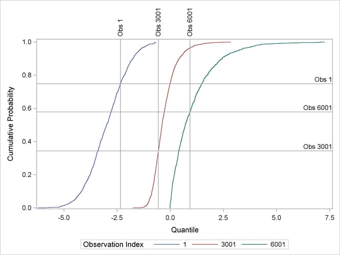
Output 96.5.5 displays the conditional CDFs for the three specified observations. Each observation has a vertical reference line for its observed response value and a horizontal reference line for its quantile level.
Output 96.5.5: Conditional Cumulative Distribution Function for Observation 1
You can also estimate the conditional probability density function (PDF) for the specified observations by using the KDE procedure. The following statements compute the probability estimates for each predicted quantile of the specified observations and plot their PDFs:
proc iml;
   use distData;
   read all var {"iObs"} into iObs;
   read all var {"qLev"} into qLev;
   read all var {"Quantiles"} into Y;
   close distData;

   nObs = &nObs;
   nTau = nrow(qLev)/nObs;
   pProb = j(nTau,3+nObs);

   pProb[,1]           = t(1:nTau);
   pProb[,2]           = qLev[1:nTau];
   pProb[1,3]          = (qLev[1]+qLev[2])/2;
   pProb[nTau,3]       = 1-(qLev[nTau-1]+qLev[nTau])/2;
   pProb[2:(nTau-1),3] = (qLev[3:nTau]-qLev[1:(nTau-2)])/2;

   do j=1 to nObs;
      jump = (j-1)*nTau;
      pProb[,(3+j)] = Y[(jump+1):(jump+nTau)];
   end;

   create probData from pProb[colname={"obs" "quantLev" "pProb"
                                       "Obs1" "Obs3001" "Obs6001"}];
   append from pProb;
   close probData;
quit;


proc kde data=probData;
   weight pProb;
   univar Obs1 Obs3001 Obs6001/ plots=densityoverlay;
run;
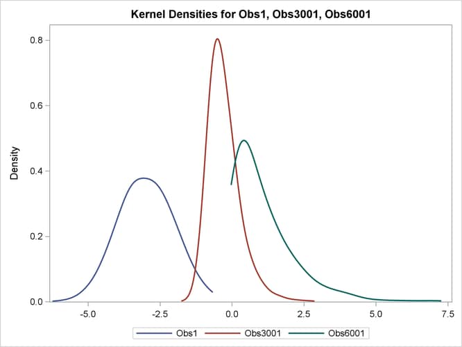
Output 96.5.6 displays the density estimation plots for the specified observations. You can see that the PDF for Observation 1 is a normal PDF, the PDF for Observation 3001 is slightly right-skewed, and the PDF for Observation 6001 is an exponential PDF.
Output 96.5.6: Density Estimates