The QUANTSELECT Procedure

Getting Started: QUANTSELECT Procedure
This example demonstrates how you can use the QUANTSELECT procedure to select covariate effects for quantile regression. The
Sashelp.Baseball data set contains salary and performance information for Major League Baseball (MLB) players, excluding pitchers, who played
at least one game in both the 1986 and 1987 seasons. The salaries (Time Inc. 1987) are for the 1987 season, and the performance measures are from 1986 (Reichler 1987).
The following step displays in Figure 96.1 the variables in the data set:
proc contents varnum data=sashelp.baseball;
   ods select position;
run;
Figure 96.1: Sashelp.Baseball Data Set
| Variables in Creation Order | ||||
|---|---|---|---|---|
| # | Variable | Type | Len | Label |
| 1 | Name | Char | 18 | Player's Name |
| 2 | Team | Char | 14 | Team at the End of 1986 |
| 3 | nAtBat | Num | 8 | Times at Bat in 1986 |
| 4 | nHits | Num | 8 | Hits in 1986 |
| 5 | nHome | Num | 8 | Home Runs in 1986 |
| 6 | nRuns | Num | 8 | Runs in 1986 |
| 7 | nRBI | Num | 8 | RBIs in 1986 |
| 8 | nBB | Num | 8 | Walks in 1986 |
| 9 | YrMajor | Num | 8 | Years in the Major Leagues |
| 10 | CrAtBat | Num | 8 | Career Times at Bat |
| 11 | CrHits | Num | 8 | Career Hits |
| 12 | CrHome | Num | 8 | Career Home Runs |
| 13 | CrRuns | Num | 8 | Career Runs |
| 14 | CrRbi | Num | 8 | Career RBIs |
| 15 | CrBB | Num | 8 | Career Walks |
| 16 | League | Char | 8 | League at the End of 1986 |
| 17 | Division | Char | 8 | Division at the End of 1986 |
| 18 | Position | Char | 8 | Position(s) in 1986 |
| 19 | nOuts | Num | 8 | Put Outs in 1986 |
| 20 | nAssts | Num | 8 | Assists in 1986 |
| 21 | nError | Num | 8 | Errors in 1986 |
| 22 | Salary | Num | 8 | 1987 Salary in $ Thousands |
| 23 | Div | Char | 16 | League and Division |
| 24 | logSalary | Num | 8 | Log Salary |
Suppose you want to investigate how the MLB players’ salaries for the 1987 season depend on performance measures for the players’
previous season and MLB careers. As a starting point for such a analysis, you can use the following statements to obtain a
parsimonious conditional median model at  :
:
proc quantselect data=sashelp.baseball;
   class Div;
   model Salary = nAtBat nHits nHome nRuns nRBI nBB yrMajor crAtBat
                  crHits crHome crRuns crRbi crBB nAssts nError nOuts
                  Div
         / selection=lasso(adaptive stop=aic choose=sbc sh=7);
run;
The SELECTION=LASSO(ADAPTIVE) option in the MODEL statement specifies the adaptive LASSO method (Zou 2006), which controls the effect selection process. The STOP=AIC option specifies that Akaike’s information criterion (AIC) be
used to determine the stopping condition. The CHOOSE=SBC option specifies that the Schwarz Bayesian information criterion
(SBC) be used to determine the final selected model. The SH=
option specifies the number of stop horizons, which requests that the selection process be stopped whenever the STOP= criterion
values at step  are worse than those for step s for some
  .
.
Figure 96.2 shows the "Model Information" table, which indicates the effect selection settings. You can see that the default quantile
type is single level, so this effect selection is effective only for .
Figure 96.2: Model Information
Figure 96.3 summarizes the effect selection process, which starts with an intercept-only model at step 0. At step 1, the effect that corresponds to the career runs is added to the model that reduced the AIC value from 2691.6511 to 2510.7297. You can see that step 10 has the minimum AIC and that step 7 has the minimum SBC. Common sense also tells you that the SBC favors a smaller model than the AIC.
Figure 96.3: Selection Summary
| Selection Summary | |||||
|---|---|---|---|---|---|
| Step | Effect Entered |
Effect Removed |
Number Effects In |
AIC | SBC |
| 0 | Intercept | 1 | 2691.6511 | 2695.2232 | |
| 1 | CrRuns | 2 | 2510.7297 | 2517.8740 | |
| 2 | nHits | 3 | 2470.4807 | 2481.1971 | |
| 3 | CrHome | 4 | 2463.5953 | 2477.8839 | |
| 4 | nBB | 5 | 2463.7806 | 2481.6414 | |
| 5 | nOuts | 6 | 2455.6212 | 2477.0541 | |
| 6 | Div AW | 7 | 2451.4609 | 2476.4660 | |
| 7 | nAtBat | 8 | 2445.0446 | 2473.6218* | |
| 8 | CrBB | 9 | 2445.5432 | 2477.6926 | |
| 9 | nHome | 10 | 2443.4818 | 2479.2033 | |
| 10 | nRuns | 11 | 2442.6036* | 2481.8973 | |
| 11 | Div NE | 12 | 2444.2409 | 2487.1067 | |
| 12 | CrAtBat | 13 | 2444.5049 | 2490.9429 | |
| 13 | Div NE | 12 | 2442.8387 | 2485.7046 | |
| 14 | YrMajor | 13 | 2443.5374 | 2489.9754 | |
| 15 | nError | 14 | 2445.2085 | 2495.2187 | |
| 16 | Div NE | 15 | 2446.4042 | 2499.9865 | |
| * Optimal Value Of Criterion | |||||
Figure 96.4 shows that the selection process stopped at a local minimum of the STOP= criterion, which is step 10. According to the SH=7 option, the effect selection process is stopped at step 10 because all the AIC values for step 11 through step 17 are no less than the AIC at step 10. Step 17 is ignored in the selection summary table because it is the last step.
Figure 96.5 shows how the final selected model is determined. CHOOSE=SBC is specified in this example, so the model at step 7 is chosen as the final selected model.
Figure 96.6 shows the final selected effects and Figure 96.7 shows the parameter estimates for the final selected model.
Figure 96.6: Selected Effects
Figure 96.7: Parameter Estimates
Quantile regression can fit a conditional quantile model at any quantile level  , so it can describe the entire distribution of a response variable conditional on covariate effects. To further investigate
the effects that might affect the MLB players’ salaries, you can also conduct effect selection at
, so it can describe the entire distribution of a response variable conditional on covariate effects. To further investigate
the effects that might affect the MLB players’ salaries, you can also conduct effect selection at  and
and  , which correspond to low-end salaries and high-end salaries respectively. The following statements use the same selection
settings that are used in the previous program:
, which correspond to low-end salaries and high-end salaries respectively. The following statements use the same selection
settings that are used in the previous program:
proc quantselect data=sashelp.baseball;
   class Div;
   model Salary = nAtBat nHits nHome nRuns nRBI nBB yrMajor crAtBat
                  crHits crHome crRuns crRbi crBB nAssts nError nOuts
                  Div
         / quantiles=0.1 0.9 selection=lasso(adaptive stop=aic choose=sbc sh=7);
run;
Figure 96.8 shows the effect selection summary with .
Figure 96.8: Selection Summary:
| Selection Summary | |||||
|---|---|---|---|---|---|
| Step | Effect Entered |
Effect Removed |
Number Effects In |
AIC | SBC |
| 0 | Intercept | 1 | 2008.3489 | 2011.9211 | |
| 1 | CrRuns | 2 | 1918.7675 | 1925.9118 | |
| 2 | nHits | 3 | 1897.2425 | 1907.9590* | |
| 3 | YrMajor | 4 | 1897.2476 | 1911.5362 | |
| 4 | CrBB | 5 | 1896.1765 | 1914.0373 | |
| 5 | nBB | 6 | 1894.1257 | 1915.5587 | |
| 6 | CrHome | 7 | 1895.6765 | 1920.6816 | |
| 7 | nAtBat | 8 | 1890.4051 | 1918.9824 | |
| 8 | nHome | 9 | 1891.3527 | 1923.5020 | |
| 9 | Div NE | 10 | 1891.7566 | 1927.4781 | |
| 10 | nRBI | 11 | 1893.7319 | 1933.0256 | |
| 11 | CrAtBat | 12 | 1893.9432 | 1936.8090 | |
| 12 | nRBI | 11 | 1891.9716 | 1931.2653 | |
| 13 | nAssts | 12 | 1888.6870 | 1931.5529 | |
| 14 | nRBI | 13 | 1890.5300 | 1936.9680 | |
| 15 | Div AE | 14 | 1889.4234 | 1939.4336 | |
| 16 | nRBI | 13 | 1887.6644* | 1934.1024 | |
| 17 | CrRbi | 14 | 1888.0966 | 1938.1068 | |
| 18 | Div AW | 15 | 1890.0322 | 1943.6145 | |
| 19 | nError | 16 | 1891.7949 | 1948.9494 | |
| 20 | nRuns | 17 | 1893.2801 | 1954.0067 | |
| 21 | nRBI | 18 | 1894.7805 | 1959.0793 | |
| 22 | CrHits | 19 | 1896.6868 | 1964.5578 | |
| * Optimal Value Of Criterion | |||||
Figure 96.9 shows the parameter estimates for the final selected model with . You can see from Figure 96.9 that low-end salaries for MLB players depend mainly on career runs and hits in 1986.
Figure 96.9: Parameter Estimates:
Figure 96.10 shows the effect selection summary with .
Figure 96.10: Selection Summary:
| Selection Summary | |||||
|---|---|---|---|---|---|
| Step | Effect Entered |
Effect Removed |
Number Effects In |
AIC | SBC |
| 0 | Intercept | 1 | 2436.7289 | 2440.3011 | |
| 1 | CrHits | 2 | 2197.4349 | 2204.5792 | |
| 2 | CrRbi | 3 | 2183.6148 | 2194.3313 | |
| 3 | nHits | 4 | 2113.2757 | 2127.5643 | |
| 4 | CrRbi | 3 | 2127.8632 | 2138.5797 | |
| 5 | CrRbi | 4 | 2113.2757 | 2127.5643 | |
| 6 | CrRbi | 3 | 2127.8632 | 2138.5797 | |
| 7 | CrRbi | 4 | 2113.2757 | 2127.5643 | |
| 8 | CrHome | 5 | 2099.2203 | 2117.0811 | |
| 9 | CrRbi | 4 | 2099.3891 | 2113.6777 | |
| 10 | CrRbi | 5 | 2099.2203 | 2117.0811 | |
| 11 | CrRbi | 4 | 2099.3891 | 2113.6777 | |
| 12 | nOuts | 5 | 2067.1926 | 2085.0533 | |
| 13 | Div AW | 6 | 2048.2393 | 2069.6723 | |
| 14 | CrRuns | 7 | 2028.8040 | 2053.8090 | |
| 15 | nAtBat | 8 | 2012.8195 | 2041.3968 | |
| 16 | CrHits | 7 | 2017.0290 | 2042.0341 | |
| 17 | CrRbi | 8 | 2009.3551 | 2037.9324 | |
| 18 | CrAtBat | 9 | 2011.2415 | 2043.3908 | |
| 19 | CrRbi | 8 | 2011.4053 | 2039.9825 | |
| 20 | CrRbi | 9 | 2011.2415 | 2043.3908 | |
| 21 | CrAtBat | 8 | 2009.3551 | 2037.9324 | |
| 22 | CrAtBat | 9 | 2011.2415 | 2043.3908 | |
| 23 | nBB | 10 | 2004.5033 | 2040.2249 | |
| 24 | CrAtBat | 9 | 2003.1023 | 2035.2517 | |
| 25 | CrAtBat | 10 | 2004.5033 | 2040.2249 | |
| 26 | CrAtBat | 9 | 2003.1023 | 2035.2517* | |
| 27 | CrAtBat | 10 | 2004.5033 | 2040.2249 | |
| 28 | nError | 11 | 2004.2230 | 2043.5167 | |
| 29 | CrHits | 12 | 2003.0544 | 2045.9203 | |
| 30 | Div NE | 13 | 2001.9603 | 2048.3983 | |
| 31 | Div AE | 14 | 2001.8349* | 2051.8451 | |
| 32 | nRuns | 15 | 2003.5961 | 2057.1784 | |
| 33 | nHome | 16 | 2004.2721 | 2061.4266 | |
| 34 | nRBI | 17 | 2006.0023 | 2066.7289 | |
| 35 | YrMajor | 18 | 2007.9975 | 2072.2963 | |
| 36 | CrBB | 19 | 2009.9514 | 2077.8223 | |
| 37 | nAssts | 20 | 2011.9095 | 2083.3525 | |
| * Optimal Value Of Criterion | |||||
Figure 96.11 shows the parameter estimates for the final selected model with .
Figure 96.11: Parameter Estimates:
| Parameter Estimates | |||
|---|---|---|---|
| Parameter | DF | Estimate | Standardized Estimate |
| Intercept | 1 | 92.893875 | 0 |
| nAtBat | 1 | -1.858170 | -0.587509 |
| nHits | 1 | 8.155573 | 0.795335 |
| nBB | 1 | 3.392794 | 0.161751 |
| CrHome | 1 | 3.191472 | 0.608700 |
| CrRuns | 1 | 1.394317 | 1.034939 |
| CrRbi | 1 | -0.913371 | -0.664951 |
| nOuts | 1 | 0.437241 | 0.271323 |
| Div AW | 1 | -167.110005 | -0.164764 |
To visually illustrate how the model evolves through the selection process, the QUANTSELECT procedure provides the coefficient
plot, the average check loss plot, and several criterion plots in either packed or unpacked forms. You can request these plots
by using the PLOTS=
option. The following statements request all the plots for the baseball data at ; they also use the STOP=AIC criterion, the CHOOSE=SBC criterion, and the SH=7 option:
ods graphics on;
proc quantselect data=sashelp.baseball plots=all;
   class Div;
   model Salary = nAtBat nHits nHome nRuns nRBI nBB yrMajor crAtBat
                  crHits crHome crRuns crRbi crBB nAssts nError nOuts
                  Div
         / quantiles=0.1 selection=lasso(adaptive stop=aic choose=sbc sh=7);
run;
Figure 96.12 shows the progression of the parameter estimates as the selection process proceeds.
Figure 96.12: Coefficient Panel:
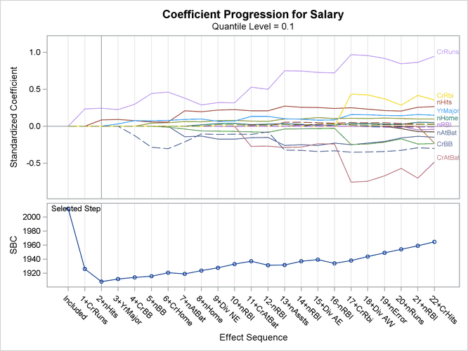
Figure 96.13 shows the progression of the average check losses as the selection process proceeds.
Figure 96.13: Average Check Loss Plot:
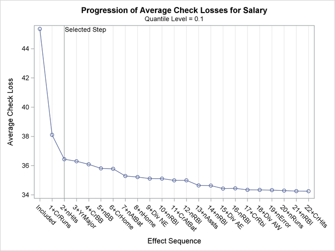
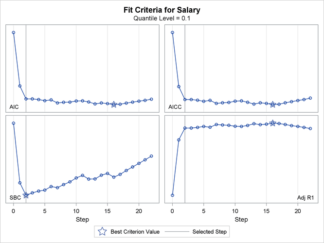
Figure 96.14 shows the progression of four effect selection criteria as the selection process proceeds.
Figure 96.14: Criterion Panel: