The PROBIT Procedure
- Overview
-
Getting Started

-
SyntaxPROC PROBIT StatementBY StatementCDFPLOT StatementCLASS StatementEFFECTPLOT StatementESTIMATE StatementINSET StatementIPPPLOT StatementLPREDPLOT StatementLSMEANS StatementLSMESTIMATE StatementMODEL StatementOUTPUT StatementPREDPPLOT StatementSLICE StatementSTORE StatementTEST StatementWEIGHT Statement
-
DetailsMissing ValuesResponse Level OrderingComputational MethodDistributionsINEST= SAS-data-setModel SpecificationLack-of-Fit TestsRescaling the Covariance MatrixTolerance DistributionInverse Confidence LimitsOUTEST= SAS-data-setXDATA= SAS-data-setTraditional High-Resolution GraphicsDisplayed OutputODS Table NamesODS Graphics
-
Examples
- References
Example 93.2 Multilevel Response
In this example, two preparations, a standard preparation and a test preparation, are each given at several dose levels to groups of insects. The symptoms are recorded for each insect within each group, and two multilevel probit models are fit. Because the natural sort order of the three levels is not the same as the response order, the ORDER=DATA response variable option is specified in the MODEL statement to get the desired order. The following statements fit two models:
data multi;
   input Prep $ Dose Symptoms $ N;
   LDose=log10(Dose);
   if Prep='test' then PrepDose=LDose;
   else PrepDose=0;
   datalines;
stand     10      None       33
stand     10      Mild        7
stand     10      Severe     10
stand     20      None       17
stand     20      Mild       13
stand     20      Severe     17
stand     30      None       14
stand     30      Mild        3
stand     30      Severe     28
stand     40      None        9
stand     40      Mild        8
stand     40      Severe     32
test      10      None       44
test      10      Mild        6
test      10      Severe      0
test      20      None       32
test      20      Mild       10
test      20      Severe     12
test      30      None       23
test      30      Mild        7
test      30      Severe     21
test      40      None       16
test      40      Mild        6
test      40      Severe     19
;
proc probit data=multi;
   class Prep;
   nonpara: model Symptoms(order=data)=Prep LDose PrepDose / lackfit;
   weight N;
run;
proc probit data=multi;
   class Prep;
   parallel: model Symptoms(order=data)=Prep LDose / lackfit;
   weight N;
run;
Results of these two models are shown in Output 93.2.1 and Output 93.2.2. The first model allows for nonparallelism between the dose response curves for the two preparations by inclusion of an interaction
between Prep and LDose. The interaction term is labeled PrepDose in the "Analysis of Parameter Estimates" table. The results of this first model indicate that the parameter for the interaction
term is not significant, having a Wald chi-square of 0.73. Also, since the first model is a generalization of the second,
a likelihood ratio test statistic for this same parameter can be obtained by multiplying the difference in log likelihoods
between the two models by 2. The value obtained,  , is 0.73. This is in close agreement with the Wald chi-square from the first model. The lack-of-fit test statistics for the
two models do not indicate a problem with either fit.
, is 0.73. This is in close agreement with the Wald chi-square from the first model. The lack-of-fit test statistics for the
two models do not indicate a problem with either fit.
Output 93.2.1: Multilevel Response: Nonparallel Analysis
| Analysis of Maximum Likelihood Parameter Estimates | ||||||||
|---|---|---|---|---|---|---|---|---|
| Parameter | DF | Estimate | Standard Error |
95% Confidence Limits | Chi-Square | Pr > ChiSq | ||
| Intercept | 1 | 3.8080 | 0.6252 | 2.5827 | 5.0333 | 37.10 | <.0001 | |
| Intercept2 | 1 | 0.4684 | 0.0559 | 0.3589 | 0.5780 | 70.19 | <.0001 | |
| Prep | stand | 1 | -1.2573 | 0.8190 | -2.8624 | 0.3479 | 2.36 | 0.1247 |
| Prep | test | 0 | 0.0000 | . | . | . | . | . |
| LDose | 1 | -2.1512 | 0.3909 | -2.9173 | -1.3851 | 30.29 | <.0001 | |
| PrepDose | 1 | -0.5072 | 0.5945 | -1.6724 | 0.6580 | 0.73 | 0.3935 | |
Output 93.2.2: Multilevel Response: Parallel Analysis
| Analysis of Maximum Likelihood Parameter Estimates | ||||||||
|---|---|---|---|---|---|---|---|---|
| Parameter | DF | Estimate | Standard Error |
95% Confidence Limits | Chi-Square | Pr > ChiSq | ||
| Intercept | 1 | 3.4148 | 0.4126 | 2.6061 | 4.2235 | 68.50 | <.0001 | |
| Intercept2 | 1 | 0.4678 | 0.0558 | 0.3584 | 0.5772 | 70.19 | <.0001 | |
| Prep | stand | 1 | -0.5675 | 0.1259 | -0.8142 | -0.3208 | 20.33 | <.0001 |
| Prep | test | 0 | 0.0000 | . | . | . | . | . |
| LDose | 1 | -2.3721 | 0.2949 | -2.9502 | -1.7940 | 64.68 | <.0001 | |
The negative coefficient associated with LDose indicates that the probability of having no symptoms (Symptoms=’None’) or no or mild symptoms (Symptoms=’None’ or Symptoms=’Mild’) decreases as LDose increases; that is, the probability of a severe symptom increases with LDose. This association is apparent for both treatment groups.
The negative coefficient associated with the standard treatment group (Prep = stand) indicates that the standard treatment is associated with more severe symptoms across all Ldose values.
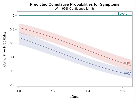
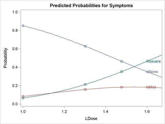
The following statements use the PLOTS= option to create the plot shown in Output 93.2.3 and Output 93.2.4. Output 93.2.3 is the plot of the probabilities of the response taking on individual levels as a function of LDose. Since there are two covariates, LDose and Prep, the value of the classification variable Prep is fixed at the highest level, test. Instead of individual response level probabilities, the CDFPLOT option creates the plot of the cumulative response probabilities
with confidence limits shown in Output 93.2.4.
proc probit data=multi
            plots=(predpplot(level=("None" "Mild" "Severe"))
                   cdfplot(level=("None" "Mild" "Severe")));
   class Prep;
   parallel: model Symptoms(order=data)=Prep LDose / lackfit;
   weight N;
run;
Output 93.2.3: Plot of Predicted Probabilities for the Test Preparation Group
Output 93.2.4: Plot of Predicted Cumulative Probabilities for the Test Preparation Group
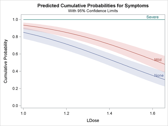
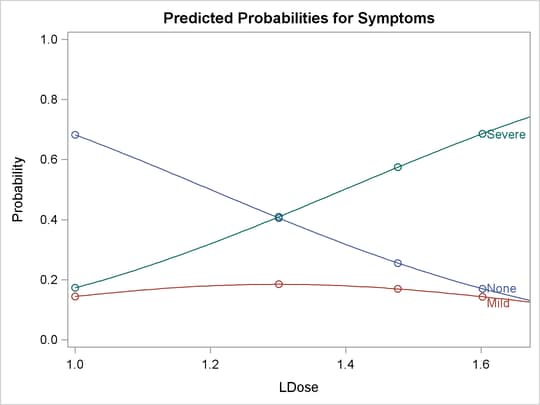
The following statements use the XDATA= data set to create plots of predicted probabilities and cumulative probabilities with
Prep set to the stand level. The resulting plots are shown in Output 93.2.5 and Output 93.2.6.
data xrow;
   input Prep $ Dose Symptoms $ N;
   LDose=log10(Dose);
   datalines;
stand     40      Severe     32
run;

proc probit data=multi xdata=xrow
            plots=(predpplot(level=("None" "Mild" "Severe"))
                   cdfplot(level=("None" "Mild" "Severe")));
   class Prep;
   parallel: model Symptoms(order=data)=Prep LDose / lackfit;
   weight N;
run;
Output 93.2.5: Plot of Predicted Probabilities for the Standard Preparation Group
Output 93.2.6: Plot of Predicted Cumulative Probabilities for the Standard Preparation Group