The PROBIT Procedure
- Overview
-
Getting Started

-
SyntaxPROC PROBIT StatementBY StatementCDFPLOT StatementCLASS StatementEFFECTPLOT StatementESTIMATE StatementINSET StatementIPPPLOT StatementLPREDPLOT StatementLSMEANS StatementLSMESTIMATE StatementMODEL StatementOUTPUT StatementPREDPPLOT StatementSLICE StatementSTORE StatementTEST StatementWEIGHT Statement
-
DetailsMissing ValuesResponse Level OrderingComputational MethodDistributionsINEST= SAS-data-setModel SpecificationLack-of-Fit TestsRescaling the Covariance MatrixTolerance DistributionInverse Confidence LimitsOUTEST= SAS-data-setXDATA= SAS-data-setTraditional High-Resolution GraphicsDisplayed OutputODS Table NamesODS Graphics
-
Examples
- References
Example 93.1 Dosage Levels
In this example, Dose is a variable representing the level of a stimulus, N represents the number of subjects tested at each level of the stimulus, and Response is the number of subjects responding to that level of the stimulus. Both probit and logit response models are fit to the
data. The LOG10 option in the PROC PROBIT statement requests that the log base 10 of Dose is used as the independent variable. Specifically, for a given level of Dose, the probability p of a positive response is modeled as
![\[ p = \Pr ({\Variable{Response}}) = F \left( b_0 + b_1 \times \log _{10}({\Variable{Dose}}) \right) \]](images/statug_probit0095.png)
The probabilities are estimated first by using the normal distribution function (the default) and then by using the logistic distribution function. Note that, in this model specification, the natural rate is assumed to be zero.
The LACKFIT option specifies lack-of-fit tests and the INVERSECL option specifies inverse confidence limits.
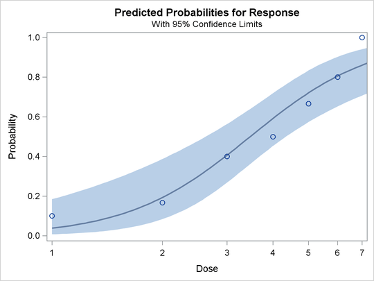
In the DATA step that reads the data, a number of observations are generated that have a missing value for the response. Although the PROBIT procedure does not use the observations with the missing values to fit the model, it does give predicted values for all nonmissing sets of independent variables. These data points fill in the plot of fitted and observed values in the logistic model displayed in Output 93.1.7. The plot, requested with the PLOT=PREDPPLOT option, displays the estimated logistic cumulative distribution function and the observed response rates.
The following statements produce Output 93.1.1:
data a;
   infile cards eof=eof;
   input Dose N Response @@;
   Observed= Response/N;
   output;
   return;
eof: do Dose=0.5 to 7.5 by 0.25;
        output;
     end;
   datalines;
1 10 1  2 12 2  3 10 4  4 10 5
5 12 8  6 10 8  7 10 10
;
ods graphics on;

proc probit log10;
   model Response/N=Dose / lackfit inversecl itprint;
   output out=B p=Prob std=std xbeta=xbeta;
run;
Output 93.1.1: Probit Analysis with Normal Distribution
| Iteration History for Parameter Estimates | ||||
|---|---|---|---|---|
| Iter | Ridge | Loglikelihood | Intercept | Log10(Dose) |
| 0 | 0 | -51.292891 | 0 | 0 |
| 1 | 0 | -37.881166 | -1.355817008 | 2.635206083 |
| 2 | 0 | -37.286169 | -1.764939171 | 3.3408954936 |
| 3 | 0 | -37.280389 | -1.812147863 | 3.4172391614 |
| 4 | 0 | -37.280388 | -1.812704962 | 3.418117919 |
| 5 | 0 | -37.280388 | -1.812704962 | 3.418117919 |
The p-values in the goodness-of-fit table of 0.6009 for the Pearson’s chi-square and 0.4616 for the likelihood ratio chi-square indicate an adequate fit for the model fit with the normal distribution.
Tolerance distribution parameter estimates for the normal distribution indicate a mean tolerance for the population of 0.5303.
Output 93.1.2 displays probit analysis with the logarithm of dose levels. The LD50 (ED50 for log dose) is 0.5303, the dose corresponding to a probability of 0.5. This is the same as the mean tolerance for the normal distribution.
Output 93.1.2: Probit Analysis with Normal Distribution
| Probit Analysis on Log10(Dose) | |||
|---|---|---|---|
| Probability | Log10(Dose) | 95% Fiducial Limits | |
| 0.01 | -0.15027 | -0.69518 | 0.07710 |
| 0.02 | -0.07052 | -0.55766 | 0.13475 |
| 0.03 | -0.01992 | -0.47064 | 0.17156 |
| 0.04 | 0.01814 | -0.40534 | 0.19941 |
| 0.05 | 0.04911 | -0.35233 | 0.22218 |
| 0.06 | 0.07546 | -0.30731 | 0.24165 |
| 0.07 | 0.09857 | -0.26793 | 0.25881 |
| 0.08 | 0.11926 | -0.23273 | 0.27425 |
| 0.09 | 0.13807 | -0.20080 | 0.28837 |
| 0.10 | 0.15539 | -0.17147 | 0.30142 |
| 0.15 | 0.22710 | -0.05086 | 0.35631 |
| 0.20 | 0.28410 | 0.04369 | 0.40124 |
| 0.25 | 0.33299 | 0.12343 | 0.44116 |
| 0.30 | 0.37690 | 0.19348 | 0.47857 |
| 0.35 | 0.41759 | 0.25658 | 0.51504 |
| 0.40 | 0.45620 | 0.31429 | 0.55182 |
| 0.45 | 0.49356 | 0.36754 | 0.58999 |
| 0.50 | 0.53032 | 0.41693 | 0.63057 |
| 0.55 | 0.56709 | 0.46296 | 0.67451 |
| 0.60 | 0.60444 | 0.50618 | 0.72271 |
| 0.65 | 0.64305 | 0.54734 | 0.77603 |
| 0.70 | 0.68374 | 0.58745 | 0.83550 |
| 0.75 | 0.72765 | 0.62776 | 0.90265 |
| 0.80 | 0.77655 | 0.66999 | 0.98008 |
| 0.85 | 0.83354 | 0.71675 | 1.07279 |
| 0.90 | 0.90525 | 0.77313 | 1.19191 |
| 0.91 | 0.92257 | 0.78646 | 1.22098 |
| 0.92 | 0.94139 | 0.80083 | 1.25265 |
| 0.93 | 0.96208 | 0.81653 | 1.28759 |
| 0.94 | 0.98519 | 0.83394 | 1.32672 |
| 0.95 | 1.01154 | 0.85367 | 1.37149 |
| 0.96 | 1.04250 | 0.87669 | 1.42424 |
| 0.97 | 1.08056 | 0.90480 | 1.48928 |
| 0.98 | 1.13116 | 0.94189 | 1.57602 |
| 0.99 | 1.21092 | 0.99987 | 1.71321 |
Output 93.1.3 displays probit analysis with dose levels. The ED50 for dose is 3.39 with a 95% confidence interval of (2.61, 4.27).
Output 93.1.3: Probit Analysis with Normal Distribution
| Probit Analysis on Dose | |||
|---|---|---|---|
| Probability | Dose | 95% Fiducial Limits | |
| 0.01 | 0.70750 | 0.20175 | 1.19427 |
| 0.02 | 0.85012 | 0.27691 | 1.36380 |
| 0.03 | 0.95517 | 0.33834 | 1.48444 |
| 0.04 | 1.04266 | 0.39324 | 1.58274 |
| 0.05 | 1.11971 | 0.44429 | 1.66793 |
| 0.06 | 1.18976 | 0.49282 | 1.74443 |
| 0.07 | 1.25478 | 0.53960 | 1.81473 |
| 0.08 | 1.31600 | 0.58515 | 1.88042 |
| 0.09 | 1.37427 | 0.62980 | 1.94252 |
| 0.10 | 1.43019 | 0.67380 | 2.00181 |
| 0.15 | 1.68696 | 0.88950 | 2.27147 |
| 0.20 | 1.92353 | 1.10584 | 2.51906 |
| 0.25 | 2.15276 | 1.32870 | 2.76161 |
| 0.30 | 2.38180 | 1.56128 | 3.01000 |
| 0.35 | 2.61573 | 1.80543 | 3.27374 |
| 0.40 | 2.85893 | 2.06200 | 3.56306 |
| 0.45 | 3.11573 | 2.33098 | 3.89038 |
| 0.50 | 3.39096 | 2.61175 | 4.27138 |
| 0.55 | 3.69051 | 2.90374 | 4.72619 |
| 0.60 | 4.02199 | 3.20759 | 5.28090 |
| 0.65 | 4.39594 | 3.52651 | 5.97077 |
| 0.70 | 4.82770 | 3.86765 | 6.84706 |
| 0.75 | 5.34134 | 4.24385 | 7.99189 |
| 0.80 | 5.97787 | 4.67724 | 9.55169 |
| 0.85 | 6.81617 | 5.20900 | 11.82480 |
| 0.90 | 8.03992 | 5.93105 | 15.55653 |
| 0.91 | 8.36704 | 6.11584 | 16.63320 |
| 0.92 | 8.73752 | 6.32165 | 17.89163 |
| 0.93 | 9.16385 | 6.55431 | 19.39034 |
| 0.94 | 9.66463 | 6.82245 | 21.21881 |
| 0.95 | 10.26925 | 7.13949 | 23.52275 |
| 0.96 | 11.02811 | 7.52816 | 26.56066 |
| 0.97 | 12.03830 | 8.03149 | 30.85201 |
| 0.98 | 13.52585 | 8.74763 | 37.67206 |
| 0.99 | 16.25233 | 9.99709 | 51.66627 |
The following statements request probit analysis of dosage levels with the logistic distribution:
proc probit log10 plot=predpplot;
   model Response/N=Dose / d=logistic inversecl;
   output out=B p=Prob std=std xbeta=xbeta;
run;
The regression parameter estimates in Output 93.1.4 for the logistic model of –3.22 and 5.97 are approximately  times as large as those for the normal model.
Output 93.1.4: Probit Analysis with Logistic Distribution
Output 93.1.5 and Output 93.1.6 show that both the ED50 and the LD50 are similar to those for the normal model.
Output 93.1.5: Probit Analysis with Logistic Distribution
| Probit Analysis on Log10(Dose) | |||
|---|---|---|---|
| Probability | Log10(Dose) | 95% Fiducial Limits | |
| 0.01 | -0.22955 | -0.97441 | 0.04234 |
| 0.02 | -0.11175 | -0.75158 | 0.12404 |
| 0.03 | -0.04212 | -0.62018 | 0.17265 |
| 0.04 | 0.00780 | -0.52618 | 0.20771 |
| 0.05 | 0.04693 | -0.45265 | 0.23533 |
| 0.06 | 0.07925 | -0.39205 | 0.25826 |
| 0.07 | 0.10686 | -0.34037 | 0.27796 |
| 0.08 | 0.13103 | -0.29521 | 0.29530 |
| 0.09 | 0.15259 | -0.25502 | 0.31085 |
| 0.10 | 0.17209 | -0.21875 | 0.32498 |
| 0.15 | 0.24958 | -0.07552 | 0.38207 |
| 0.20 | 0.30792 | 0.03092 | 0.42645 |
| 0.25 | 0.35611 | 0.11742 | 0.46451 |
| 0.30 | 0.39820 | 0.19143 | 0.49932 |
| 0.35 | 0.43644 | 0.25684 | 0.53275 |
| 0.40 | 0.47221 | 0.31588 | 0.56619 |
| 0.45 | 0.50651 | 0.36986 | 0.60089 |
| 0.50 | 0.54013 | 0.41957 | 0.63807 |
| 0.55 | 0.57374 | 0.46559 | 0.67894 |
| 0.60 | 0.60804 | 0.50846 | 0.72474 |
| 0.65 | 0.64381 | 0.54896 | 0.77673 |
| 0.70 | 0.68205 | 0.58815 | 0.83637 |
| 0.75 | 0.72414 | 0.62752 | 0.90582 |
| 0.80 | 0.77233 | 0.66915 | 0.98876 |
| 0.85 | 0.83067 | 0.71631 | 1.09242 |
| 0.90 | 0.90816 | 0.77562 | 1.23343 |
| 0.91 | 0.92766 | 0.79014 | 1.26931 |
| 0.92 | 0.94922 | 0.80607 | 1.30912 |
| 0.93 | 0.97339 | 0.82378 | 1.35391 |
| 0.94 | 1.00100 | 0.84384 | 1.40523 |
| 0.95 | 1.03332 | 0.86713 | 1.46546 |
| 0.96 | 1.07245 | 0.89511 | 1.53864 |
| 0.97 | 1.12237 | 0.93053 | 1.63228 |
| 0.98 | 1.19200 | 0.97952 | 1.76329 |
| 0.99 | 1.30980 | 1.06166 | 1.98569 |
Output 93.1.6: Probit Analysis with Logistic Distribution
| Probit Analysis on Dose | |||
|---|---|---|---|
| Probability | Dose | 95% Fiducial Limits | |
| 0.01 | 0.58945 | 0.10607 | 1.10241 |
| 0.02 | 0.77312 | 0.17718 | 1.33058 |
| 0.03 | 0.90757 | 0.23978 | 1.48817 |
| 0.04 | 1.01813 | 0.29773 | 1.61327 |
| 0.05 | 1.11413 | 0.35266 | 1.71922 |
| 0.06 | 1.20018 | 0.40546 | 1.81244 |
| 0.07 | 1.27896 | 0.45670 | 1.89654 |
| 0.08 | 1.35218 | 0.50675 | 1.97379 |
| 0.09 | 1.42100 | 0.55588 | 2.04572 |
| 0.10 | 1.48625 | 0.60430 | 2.11339 |
| 0.15 | 1.77656 | 0.84038 | 2.41030 |
| 0.20 | 2.03199 | 1.07379 | 2.66961 |
| 0.25 | 2.27043 | 1.31046 | 2.91416 |
| 0.30 | 2.50152 | 1.55393 | 3.15736 |
| 0.35 | 2.73172 | 1.80652 | 3.40996 |
| 0.40 | 2.96627 | 2.06957 | 3.68292 |
| 0.45 | 3.21006 | 2.34345 | 3.98927 |
| 0.50 | 3.46837 | 2.62768 | 4.34578 |
| 0.55 | 3.74746 | 2.92138 | 4.77466 |
| 0.60 | 4.05546 | 3.22451 | 5.30573 |
| 0.65 | 4.40366 | 3.53961 | 5.98041 |
| 0.70 | 4.80891 | 3.87391 | 6.86079 |
| 0.75 | 5.29836 | 4.24155 | 8.05044 |
| 0.80 | 5.92009 | 4.66820 | 9.74455 |
| 0.85 | 6.77126 | 5.20365 | 12.37149 |
| 0.90 | 8.09391 | 5.96508 | 17.11715 |
| 0.91 | 8.46559 | 6.16800 | 18.59129 |
| 0.92 | 8.89644 | 6.39837 | 20.37592 |
| 0.93 | 9.40575 | 6.66469 | 22.58957 |
| 0.94 | 10.02317 | 6.97977 | 25.42292 |
| 0.95 | 10.79732 | 7.36428 | 29.20549 |
| 0.96 | 11.81534 | 7.85438 | 34.56521 |
| 0.97 | 13.25466 | 8.52173 | 42.88232 |
| 0.98 | 15.55972 | 9.53941 | 57.98207 |
| 0.99 | 20.40815 | 11.52549 | 96.75820 |
The PLOT=PREDPPLOT option together with the ODS GRAPHICS statement creates the plot of observed and fitted probabilities in Output 93.1.7. The dashed line represent pointwise confidence bands for the probabilities.
Output 93.1.7: Plot of Observed and Fitted Probabilities