The ICPHREG Procedure

Baseline Parameterization
Because any one of the baseline hazard, cumulative hazard, and survival functions determines the others, it is sufficient to parameterize one of them. For the baseline function, PROC ICPHREG supports the parameterizations that are described in the following subsections.
Piecewise Constant Model
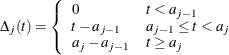
As its name suggests, the piecewise constant hazard rate model parameterizes the baseline hazard function as a union of several disjoint intervals, within each of which the hazard rate is constant:
![\[ \lambda _0(t)= r_ j ~ ~ \mr{if}~ a_{j-1} \le t < a_ j, j=1,\ldots ,J \]](images/statug_icphreg0064.png)
It follows that the baseline cumulative hazard function is
![\[ \Lambda _0(t)= \sum _{j=1}^ J r_ j \Delta _ j(t) \]](images/statug_icphreg0065.png)
where
To produce a meaningful hazard function, the  need to be bounded below by 0. Such a constraint can be removed by transforming the parameters to a natural log scale:
![\[ \alpha _ j=\log (r_ j), \mbox{~ ~ } j=1,\ldots ,J \]](images/statug_icphreg0068.png)
PROC ICPHREG uses either the original or the transformed scale to fit piecewise constant models. You can change the scale by using the HAZSCALE= option. By default, the original scale is used.
Cubic Splines Model
For the proportional hazards model, Royston and Parmar (2002) propose modeling the log of the baseline cumulative hazard function in terms of natural cubic splines,
![\[ \log [\Lambda _0(t)] = \gamma _0 + \gamma _1 x + \gamma _2 v_1(x) + \cdots + \gamma _{m+1} v_ J(x) \]](images/statug_icphreg0069.png)
where  represents the time on a log scale. The
  are the basis functions, which are computed as
![\[ v_ j(x) = (x-k_ j)_+^3 - e_ j (x-k_{\mr{min}})_+^3 - (1-e_ j) (x-k_{\mr{max}})_+^3 \]](images/statug_icphreg0072.png)
where
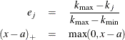
Here,  and
and  are two terminal knots, and
  are m interval knots that are placed between and . The degrees of freedom equals
  . When
  , the log of the baseline hazard becomes
  , which corresponds to a common form of the
Weibull model. When
, which corresponds to a common form of the
Weibull model. When  , the Weibull model further reduces to the exponential model.