The FMM Procedure

Metropolis-Hastings Algorithm
If Metropolis-Hastings is the only sampler available for the specified model (see Table 39.8) or if the METROPOLIS option is specified in the BAYES statement, PROC FMM uses the Metropolis-Hastings approach of Gamerman (1997). See the section Metropolis and Metropolis-Hastings Algorithms in Chapter 7: Introduction to Bayesian Analysis Procedures, for a general discussion of the Metropolis-Hastings algorithm.
The Gamerman (1997) algorithm derives a specific density that is used to generate proposals for the component-specific parameters  . The form of this proposal density is multivariate normal, with mean
  and covariance matrix
  derived as follows.
Suppose is the vector of model coefficients in the jth component and suppose that has prior distribution  . Consider a generalized linear model (GLM) with link function
  and variance function
  . The pseudo-response and weight in the GLM for a weighted least squares step are
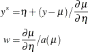
If the model contains offsets or FREQ or WEIGHT statements, or if a trials variable is involved, suitable adjustments are made to these quantities.
In each component,  , form an adjusted cross-product matrix with a "pseudo" border
![\[ \left[ \begin{array}{ll} \bX _ j’\bW _ j\bX _ j + \bR ^{-1} & \bX _ j’\bW _ j\mb{y}_ j^* + \bR ^{-1}\mb{a} \cr \mb{y}_ j^{*'}\bW _ j\bX _ j + \mb{a}’\bR ^{-1} & c \end{array}\right] \]](images/statug_fmm0295.png)
where  is a diagonal matrix formed from the pseudo-weights w,
  is a vector of pseudo-responses, and c is arbitrary. This is basically a system of normal equations with ridging, and the degree of ridging is governed by the precision
and mean of the normal prior distribution of the coefficients. Sweeping on the leading partition leads to
is a vector of pseudo-responses, and c is arbitrary. This is basically a system of normal equations with ridging, and the degree of ridging is governed by the precision
and mean of the normal prior distribution of the coefficients. Sweeping on the leading partition leads to
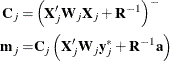
where the generalized inverse is a reflexive,  -inverse (see the section Linear Model Theory in Chapter 3: Introduction to Statistical Modeling with SAS/STAT Software, for details).
PROC FMM then generates a proposed parameter vector from the resulting multivariate normal distribution, and then accepts or rejects this proposal according to the appropriate Metropolis-Hastings thresholds.