The FMM Procedure

Looking for Multiple Modes: Are Galaxies Clustered?
Mixture modeling is essentially a generalized form of one-dimensional cluster analysis. The following example shows how you can use PROC FMM to explore the number and nature of Gaussian clusters in univariate data.
Roeder (1990) presents data from the Corona Borealis sky survey with the velocities of 82 galaxies in a narrow slice of the sky. Cosmological theory suggests that the observed velocity of each galaxy is proportional to its distance from the observer. Thus, the presence of multiple modes in the density of these velocities could indicate a clustering of the galaxies at different distances.
The following DATA step recreates the data set in Roeder (1990). The computed variable v represents the measured velocity in thousands of kilometers per second.
title "FMM Analysis of Galaxies Data";
data galaxies;
   input velocity @@;
   v = velocity / 1000;
   datalines;
9172  9350  9483  9558  9775  10227 10406 16084 16170 18419
18552 18600 18927 19052 19070 19330 19343 19349 19440 19473
19529 19541 19547 19663 19846 19856 19863 19914 19918 19973
19989 20166 20175 20179 20196 20215 20221 20415 20629 20795
20821 20846 20875 20986 21137 21492 21701 21814 21921 21960
22185 22209 22242 22249 22314 22374 22495 22746 22747 22888
22914 23206 23241 23263 23484 23538 23542 23666 23706 23711
24129 24285 24289 24366 24717 24990 25633 26960 26995 32065
32789 34279
;
Analysis of potentially multi-modal data is a natural application of finite mixture models. In this case, the modeling is complicated by the question of the variance for each of the components. Using identical variances for each component could obscure underlying structure, but the additional flexibility granted by component-specific variances might introduce spurious features.
You can use PROC FMM to prepare analyses for equal and unequal variances and use one of the available fit statistics to compare the resulting models. You can use the model selection facility to explore models that have varying numbers of mixture components—say, from three to seven as investigated in Roeder (1990). The following statements select the best unequal-variance model by using Akaike’s information criterion (AIC), which has a built-in penalty for model complexity:
title2 "Three to Seven Components, Unequal Variances";
ods graphics on;
proc fmm data=galaxies criterion=AIC;
   model v = / kmin=3 kmax=7;
run;
The KMIN= and KMAX= options indicate the smallest and largest number of components to consider. Figure 39.14, Figure 39.15, and Figure 39.16 show a selection of the output from this unequal variances model.
Figure 39.14: Model Selection for Galaxy Data Assuming Unequal Variances
| FMM Analysis of Galaxies Data |
| Three to Seven Components, Unequal Variances |
| Model Information | |
|---|---|
| Data Set | WORK.GALAXIES |
| Response Variable | v |
| Type of Model | Homogeneous Mixture |
| Distribution | Normal |
| Min Components | 3 |
| Max Components | 7 |
| Link Function | Identity |
| Estimation Method | Maximum Likelihood |
| Component Evaluation for Mixture Models | ||||||||||
|---|---|---|---|---|---|---|---|---|---|---|
| Model ID |
Number of | -2 Log L | AIC | AICC | BIC | Pearson | Max Gradient |
|||
| Components | Parameters | |||||||||
| Total | Eff. | Total | Eff. | |||||||
| 1 | 3 | 3 | 8 | 8 | 406.96 | 422.96 | 424.94 | 442.22 | 82.00 | 0.000024 |
| 2 | 4 | 4 | 11 | 11 | 406.96 | 428.96 | 432.74 | 455.44 | 82.00 | 0.00012 |
| 3 | 5 | 5 | 14 | 14 | 406.96 | 434.96 | 441.23 | 468.66 | 82.00 | 0.000050 |
| 4 | 6 | 6 | 17 | 17 | 406.96 | 440.96 | 450.53 | 481.88 | 82.00 | 0.000057 |
| 5 | 7 | 7 | 20 | 20 | 406.96 | 446.96 | 460.73 | 495.10 | 82.00 | 0.000039 |
| The model with 3 components (ID=1) was selected as 'best' based on the AIC statistic. |
Figure 39.15: Density Plot for Best (Three-Component) Model Assuming Unequal Variances
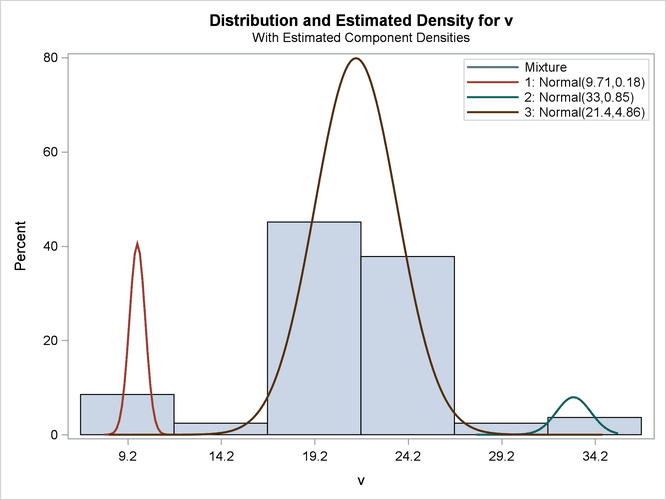
Figure 39.16: Criterion Panel Plot for Model Selection Assuming Unequal Variances
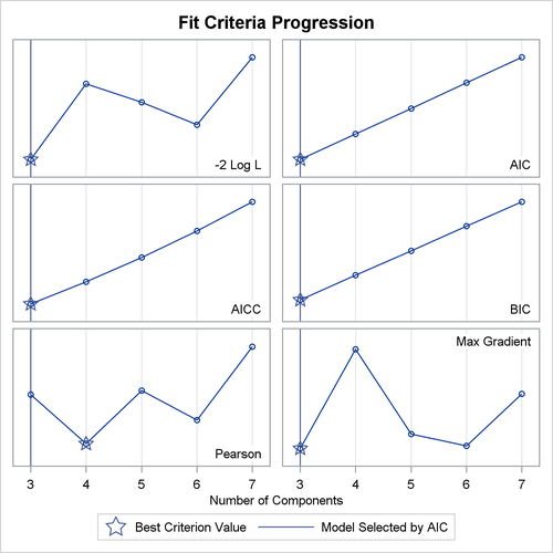
This example uses the AIC for model selection. Figure 39.16 shows the AIC and other model fit criteria for each of the fitted models.
To require that the separate components have identical variances, add the EQUATE=SCALE option in the MODEL statement:
title2 "Three to Seven Components, Equal Variances";
proc fmm data=galaxies criterion=AIC gconv=0;
   model v = / kmin=3 kmax=7  equate=scale;
run;
The GCONV= convergence criterion is turned off in this PROC FMM run to avoid the early stoppage of the iterations when the relative gradient changes little between iterations. Turning the criterion off usually ensures that convergence is achieved with a small absolute gradient of the objective function.
The output for equal variances is shown in Figure 39.17 and Figure 39.18.
Figure 39.17: Model Selection for Galaxy Data Assuming Equal Variances
| Component Evaluation for Mixture Models | ||||||||||
|---|---|---|---|---|---|---|---|---|---|---|
| Model ID |
Number of | -2 Log L | AIC | AICC | BIC | Pearson | Max Gradient |
|||
| Components | Parameters | |||||||||
| Total | Eff. | Total | Eff. | |||||||
| 1 | 3 | 3 | 6 | 6 | 478.74 | 490.74 | 491.86 | 505.18 | 82.00 | 1.197E-6 |
| 2 | 4 | 4 | 8 | 8 | 416.49 | 432.49 | 434.47 | 451.75 | 82.00 | 6.161E-6 |
| 3 | 5 | 5 | 10 | 10 | 416.49 | 436.49 | 439.59 | 460.56 | 82.00 | 4.316E-6 |
| 4 | 6 | 6 | 12 | 12 | 416.49 | 440.49 | 445.02 | 469.37 | 82.00 | 6.294E-6 |
| 5 | 7 | 7 | 14 | 14 | 416.49 | 444.49 | 450.76 | 478.19 | 82.00 | 4.884E-6 |
| The model with 4 components (ID=2) was selected as 'best' based on the AIC statistic. |
| Parameter Estimates for Normal Model | |||||
|---|---|---|---|---|---|
| Component | Parameter | Estimate | Standard Error |
z Value | Pr > |z| |
| 1 | Intercept | 23.5058 | 0.3460 | 67.93 | <.0001 |
| 2 | Intercept | 33.0440 | 0.7610 | 43.42 | <.0001 |
| 3 | Intercept | 20.0086 | 0.3029 | 66.06 | <.0001 |
| 4 | Intercept | 9.7103 | 0.4981 | 19.50 | <.0001 |
| 1 | Variance | 1.7354 | 0.3905 | ||
| 2 | Variance | 1.7354 | 0.3905 | ||
| 3 | Variance | 1.7354 | 0.3905 | ||
| 4 | Variance | 1.7354 | 0.3905 | ||
Figure 39.18: Density Plot for Best (Four-Component) Model Assuming Equal Variances
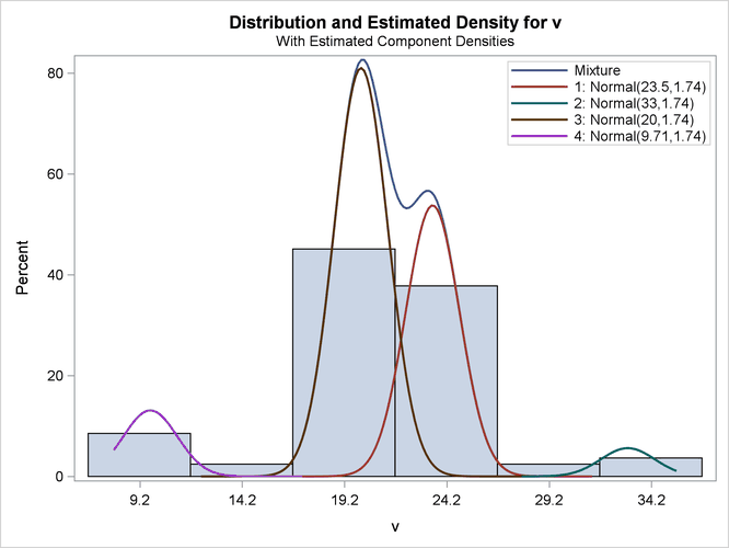
Not surprisingly, the two variance specifications produce different optimal models. The unequal variance specification favors a three-component model while the equal variance specification favors a four-component model. Comparison of the AIC fit statistics, 423.0 and 432.5, indicates that the three-component, unequal variance model provides the best overall fit.