The FMM Procedure

Example 39.3 Enforcing Homogeneity Constraints: Count and Dispersion—It Is All Over!
The following example demonstrates how you can use either the EQUATE= option in the MODEL statement or the RESTRICT statement to impose homogeneity constraints on chosen model effects.
The data for this example were presented by Margolin, Kaplan, and Zeiger (1981) and analyzed by various authors applying a number of techniques. The following DATA step shows the number of revertant salmonella
colonies (variable num) at six levels of quinoline dosing (variable dose). There are three replicate plates at each dose of quinoline.
data assay;
   label dose = 'Dose of quinoline (microg/plate)'
         num  = 'Observed number of colonies';
   input dose @;
   logd = log(dose+10);
   do i=1 to 3; input num@; output; end;
   datalines;
   0  15 21 29
  10  16 18 21
  33  16 26 33
 100  27 41 60
 333  33 38 41
1000  20 27 42
;
The basic notion is that the data are overdispersed relative to a Poisson distribution in which the logarithm of the mean
count is modeled as a linear regression in dose (in  plate) and in the derived variable
  (Lawless 1987). The log of the expected count of revertants is thus
![\[ \beta _0 + \beta _1\mr{dose} + \beta _2\log \{ \mr{dose}+10\} \]](images/statug_fmm0376.png)
The following statements fit a standard Poisson regression model to these data:
proc fmm data=assay;
   model num = dose logd / dist=Poisson;
run;
The Pearson statistic for this model is rather large compared to the number of degrees of freedom ( ). The ratio
 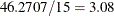 indicates an overdispersion problem in the Poisson model (Output 39.3.1).
Output 39.3.1: Result of Fitting Poisson Regression Models
Breslow (1984) accounts for overdispersion by including a random effect in the predictor for the log rate and applying a quasi-likelihood technique to estimate the parameters. Wang et al. (1996) examine these data using mixtures of Poisson regression models. They fit several two- and three-component Poisson regression mixtures. Examining the log likelihoods, AIC, and BIC criteria, they eventually settle on a two-component model in which the intercepts vary by category and the regression coefficients are the same. This mixture model can be written as
![\begin{align*} f(y) =& \pi \frac{1}{y!}\lambda _1^ y\exp \{ -\lambda _1\} + (1-\pi ) \frac{1}{y!}\lambda _2^ y\exp \{ -\lambda _2\} \\ \lambda _1 =& \exp \{ \beta _{01} + \beta _{1}\mr{dose} + \beta _2 \log [\mr{dose}+10 ] \} \\ \lambda _2 =& \exp \{ \beta _{02} + \beta _{1}\mr{dose} + \beta _2\log [ \mr{dose}+10 ] \} \\ \end{align*}](images/statug_fmm0379.png)
This model is fit with the FMM procedure with the following statements:
proc fmm data=assay;
   model num = dose logd / dist=Poisson k=2
                           equate=effects(dose logd);
run;
The EQUATE=
option in the MODEL
statement places constraints on the optimization and makes the coefficients for dose and logd homogeneous across components in the model. Output 39.3.2 displays the "Fit Statistics" and parameter estimates in the mixture. The Pearson statistic is drastically reduced compared
to the Poisson regression model in Output 39.3.1. With  degrees of freedom, the ratio of the Pearson and the degrees of freedom is now
 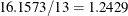 . Note that the effective number of parameters was used to compute the degrees of freedom, not the total number of parameters,
because of the equality constraints.
. Note that the effective number of parameters was used to compute the degrees of freedom, not the total number of parameters,
because of the equality constraints.
Output 39.3.2: Result for Two-Component Poisson Regression Mixture
| Parameter Estimates for Poisson Model | |||||
|---|---|---|---|---|---|
| Component | Effect | Estimate | Standard Error |
z Value | Pr > |z| |
| 1 | Intercept | 1.9097 | 0.2654 | 7.20 | <.0001 |
| 1 | dose | -0.00126 | 0.000273 | -4.62 | <.0001 |
| 1 | logd | 0.3639 | 0.06602 | 5.51 | <.0001 |
| 2 | Intercept | 2.4770 | 0.2731 | 9.07 | <.0001 |
| 2 | dose | -0.00126 | 0.000273 | -4.62 | <.0001 |
| 2 | logd | 0.3639 | 0.06602 | 5.51 | <.0001 |
You could also have used RESTRICT statements to impose the homogeneity constraints on the model fit, as shown in the following statements:
proc fmm data=assay;
   model num = dose logd / dist=Poisson k=2;
   restrict 'common dose' dose 1, dose -1;
   restrict 'common logd' logd 1, logd -1;
run;
The first RESTRICT
statement equates the coefficients for the dose variable in the two components, and the second RESTRICT
statement accomplishes the same for the coefficients of the logd variable. If the right-hand side of a restriction is not specified, PROC FMM defaults to equating the left-hand side of the
restriction to zero. The "Linear Constraints" table in Output 39.3.3 shows that both linear equality constraints are active. The parameter estimates match the previous FMM run.
Output 39.3.3: Result for Two-Component Mixture with RESTRICT Statements
| Parameter Estimates for Poisson Model | |||||
|---|---|---|---|---|---|
| Component | Effect | Estimate | Standard Error |
z Value | Pr > |z| |
| 1 | Intercept | 1.9097 | 0.2654 | 7.20 | <.0001 |
| 1 | dose | -0.00126 | 0.000273 | -4.62 | <.0001 |
| 1 | logd | 0.3639 | 0.06602 | 5.51 | <.0001 |
| 2 | Intercept | 2.4770 | 0.2731 | 9.07 | <.0001 |
| 2 | dose | -0.00126 | 0.000273 | -4.62 | <.0001 |
| 2 | logd | 0.3639 | 0.06602 | 5.51 | <.0001 |
Wang et al. (1996) note that observation 12 with a revertant colony count of 60 is comparably high. The following statements remove the observation
from the analysis and fit their selected model:
proc fmm data=assay(where=(num ne 60));
   model num = dose logd / dist=Poisson k=2
                           equate=effects(dose logd);
run;
Output 39.3.4: Result for Two-Component Model without Outlier
| Parameter Estimates for Poisson Model | |||||
|---|---|---|---|---|---|
| Component | Effect | Estimate | Standard Error |
z Value | Pr > |z| |
| 1 | Intercept | 2.2272 | 0.3022 | 7.37 | <.0001 |
| 1 | dose | -0.00065 | 0.000445 | -1.46 | 0.1440 |
| 1 | logd | 0.2432 | 0.1045 | 2.33 | 0.0199 |
| 2 | Intercept | 2.5477 | 0.3331 | 7.65 | <.0001 |
| 2 | dose | -0.00065 | 0.000445 | -1.46 | 0.1440 |
| 2 | logd | 0.2432 | 0.1045 | 2.33 | 0.0199 |
The ratio of Pearson Statistic over degrees of freedom (12) is only slightly worse than in the previous model; the loss of 5% of the observations carries a price (Output 39.3.4). The parameter estimates for the two intercepts are now fairly close. If the intercepts were identical, then the two-component model would collapse to the Poisson regression model:
proc fmm data=assay(where=(num ne 60));
   model num = dose logd / dist=Poisson;
run;
Output 39.3.5: Result of Fitting Poisson Regression Model without Outlier
Compared to the same model applied to the full data, the Pearson statistic is much reduced (compare 46.2707 in Output 39.3.1 to 27.8008 in Output 39.3.5). The outlier—or overcount, if you will—induces at least some of the overdispersion.