The FMM Procedure

Example 39.1 Modeling Mixing Probabilities: All Mice Are Created Equal, but Some Are More Equal
This example demonstrates how you can model the means and mixture proportions separately in a binomial cluster model. It also compares the binomial cluster model to the beta-binomial model.
In a typical teratological experiment, the offspring of animals that were exposed to a toxin during pregnancy are studied for malformation. If you count the number of malformed offspring in a litter of size n, then this count is typically not binomially distributed. The responses of the offspring from the same litter are not independent; hence their sum does not constitute a binomial random variable. Relative to a binomial model, data from teratological experiments exhibit overdispersion because ignoring positive correlation among the responses tends to overstate the precision of the parameter estimates. Overdispersion mechanisms are briefly discussed in the section Overdispersion.
In this application, the focus is on mixtures and models that involve a mixing mechanism. The mixing approach (Williams 1975; Haseman and Kupper 1979) supposes that the binomial success probability is a random variable that follows a  distribution:
![\begin{align*} Y|\mu & \sim \mr{Binomial}(n,\mu ) \\ \mu & \sim \mr{Beta}(\alpha ,\beta ) \\ Y & \sim \mr{Beta}\mbox{-}\mr{binomial}(n,\mu ,\phi ) \\ \mr{E}[Y] & = n\pi \\ \mr{Var}[Y] & = n\pi (1-\pi )\left\{ 1+\mu ^2(n-1)\right\} \end{align*}](images/statug_fmm0345.png)
If  , then the beta-binomial distribution reduces to a standard binomial model with success probability
  . The parameterization of the beta-binomial distribution used by the FMM procedure is based on Neerchal and Morel (1998), see the section Log-Likelihood Functions for Response Distributions for details.
Morel and Nagaraj (1993); Morel and Neerchal (1997); Neerchal and Morel (1998) propose a different model to capture dependency within binomial clusters. Their model is a two-component mixture that gives
rise to the same mean and variance function as the beta-binomial model. The genesis is different, however. In the binomial
cluster model of Morel and Neerchal, suppose there is a cluster of n Bernoulli outcomes with success probability . The number of responses in the cluster decomposes into  outcomes that all respond with either "success" or "failure"; the important aspect is that they all respond identically.
The remaining n – N Bernoulli outcomes respond independently, so the sum of successes in this group is a binomial
outcomes that all respond with either "success" or "failure"; the important aspect is that they all respond identically.
The remaining n – N Bernoulli outcomes respond independently, so the sum of successes in this group is a binomial random variable. Denote the probability with which cluster members fall into the group of identical respondents as
  . Then
  is the probability that a response belongs to the group of independent Bernoulli outcomes.
It is easy to see how this process of dividing the individual Bernoulli outcomes creates clustering. The binomial cluster model can be written as the two-component mixture
![\[ \Pr (Y = y) = \pi \Pr (U = y) + (1-\pi )\Pr (V = y) \]](images/statug_fmm0350.png)
where 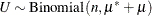 ,
, 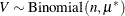 , and
, and  . This mixture model is somewhat unusual because the mixing probability appears as a parameter in the component distributions. The two probabilities involved, and , have the following interpretation: is the unconditional probability of success for any observation, and is the probability with which the Bernoulli observations respond identically. The complement of this probability, , is the probability with which the Bernoulli outcomes respond independently. If , then the two-component mixture reduces to a standard binomial model that has success probability . Because both and are involved in the success probabilities of the two binomial variables in the mixture, you can affect these binomial means
by specifying effects in the PROBMODEL
statement (for the ’s) or the MODEL
statement (for the ’s). You would vary the success probabilities
. This mixture model is somewhat unusual because the mixing probability appears as a parameter in the component distributions. The two probabilities involved, and , have the following interpretation: is the unconditional probability of success for any observation, and is the probability with which the Bernoulli observations respond identically. The complement of this probability, , is the probability with which the Bernoulli outcomes respond independently. If , then the two-component mixture reduces to a standard binomial model that has success probability . Because both and are involved in the success probabilities of the two binomial variables in the mixture, you can affect these binomial means
by specifying effects in the PROBMODEL
statement (for the ’s) or the MODEL
statement (for the ’s). You would vary the success probabilities  and
and  by using the MODEL
statement in a "straight" two-component binomial mixture,
by using the MODEL
statement in a "straight" two-component binomial mixture,
![\[ \pi \mr{Binomial}(n,\mu _1) + (1-\pi )\mr{Binomial}(n,\mu _2) \]](images/statug_fmm0356.png)
You can fit the beta-binomial model by specifying DIST= BETABIN and the binomial cluster model by specifying DIST= BINOMCLUSTER in the MODEL statement.
Morel and Neerchal (1997) report data from a completely randomized design that studies the teratogenicity of phenytoin in 81 pregnant mice. The treatment structure of the experiment is an augmented factorial. In addition to an untreated control, mice received 60 mg/kg of phenytoin (PHT), 100 mg/kg of trichloropropene oxide (TCPO), and their combination. The design was augmented with a control group that was treated with water. As in Morel and Neerchal (1997), the two control groups are combined here into a single group.
The following DATA step creates the data for this analysis as displayed in Table 1 of Morel and Neerchal (1997). The second DATA step creates continuous variables x1–x3 to match the parameterization of these authors.
data ossi;
   length tx $8;
   input tx$ n @@;
   do i=1 to n;
      input y m @@;
      output;
   end;
   drop i;
   datalines;
Control  18 8 8 9  9  7  9 0  5 3  3 5 8 9 10 5 8 5 8 1 6 0 5
            8 8 9 10  5  5 4  7 9 10 6 6 3  5
Control  17 8 9 7 10 10 10 1  6 6  6 1 9 8  9 6 7 5 5 7 9
            2 5 5  6  2  8 1  8 0  2 7 8 5  7
PHT      19 1 9 4  9  3  7 4  7 0  7 0 4 1  8 1 7 2 7 2 8 1 7
            0 2 3 10  3  7 2  7 0  8 0 8 1 10 1 1
TCPO     16 0 5 7 10  4  4 8 11 6 10 6 9 3  4 2 8 0 6 0 9
            3 6 2  9  7  9 1 10 8  8 6 9
PHT+TCPO 11 2 2 0  7  1  8 7  8 0 10 0 4 0  6 0 7 6 6 1 6 1 7
;

data ossi;
   set ossi;
   array xx{3} x1-x3;
   do i=1 to 3; xx{i}=0; end;
   pht  = 0;
   tcpo = 0;
   if (tx='TCPO') then do;
      xx{1} = 1;
      tcpo  = 100;
   end; else if (tx='PHT') then do;
      xx{2} = 1;
      pht   = 60;
   end; else if (tx='PHT+TCPO') then do;
      pht  = 60;
      tcpo = 100;
      xx{1} = 1; xx{2} = 1; xx{3}=1;
   end;
run;
The FMM procedure models the mean parameters through the MODEL
statement and the mixing proportions through the PROBMODEL
statement. In the binomial cluster model, you can place a regression structure on either set of probabilities, and the regression
structure does not need to be the same. In the following statements, the unconditional probability of ossification is modeled
as a two-way factorial, whereas the intralitter effect—the propensity to group within a cluster—is assumed to be constant:
proc fmm data=ossi;
   class pht tcpo;
   model y/m = / dist=binomcluster;
   probmodel pht tcpo pht*tcpo;
run;
The CLASS
statement declares the PHT and TCPO variables as classification variables. They affect the analysis through their levels, not through their numeric values. The
MODEL
statement declares the distribution of the data to follow a binomial cluster model. The FMM procedure then automatically
assumes that the model is a two-component mixture. An intercept is included by default. The PROBMODEL
statement declares the effect structure for the mixing probabilities. The unconditional probability of ossification of a
fetus depends on the main effects and the interaction in the factorial.
The "Model Information" table displays important details about the model fit with the FMM procedure (Output 39.1.1). Although no K=
option was specified in the MODEL
statement, the FMM procedure recognizes the model as a two-component model. The "Class Level Information" table displays
the levels and values of the PHT and TCPO variables. Eighty-one observations are read from the data and are used in the analysis. These observations comprise 287 events
and 585 total outcomes.
Output 39.1.1: Model Information in Binomial Cluster Model with Constant Clustering Probability
The "Optimization Information" table in Output 39.1.2 gives details about the maximum likelihood optimization. By default, the FMM procedure uses a quasi-Newton algorithm. The
model contains five parameters, four of which are part of the model for the mixing probabilities. The fifth parameter is the
intercept in the model for .
Output 39.1.2: Optimization in Binomial Cluster Model with Constant Clustering Probability
| Iteration History | ||||
|---|---|---|---|---|
| Iteration | Evaluations | Objective Function |
Change | Max Gradient |
| 0 | 5 | 174.92723892 | . | 43.78769 |
| 1 | 2 | 154.13180744 | 20.79543149 | 11.2346 |
| 2 | 3 | 153.26693611 | 0.86487133 | 6.888215 |
| 3 | 2 | 152.84974281 | 0.41719329 | 3.541977 |
| 4 | 3 | 152.61756033 | 0.23218248 | 2.783556 |
| 5 | 3 | 152.54795303 | 0.06960730 | 1.146807 |
| 6 | 3 | 152.52684929 | 0.02110374 | 0.034367 |
| 7 | 3 | 152.52671214 | 0.00013715 | 0.011511 |
| 8 | 3 | 152.52670799 | 0.00000415 | 0.000202 |
| 9 | 3 | 152.52670799 | 0.00000000 | 4.001E-6 |
After nine iterations, the iterative optimization converges. The –2 log likelihood at the converged solution is 305.1, and the Pearson statistic is 89.2077. The FMM procedure computes the Pearson statistic as a general goodness-of-fit measure that expresses the closeness of the fitted model to the data.
The estimates of the parameters in the conditional probability and in the unconditional probability are given in Output 39.1.3. The intercept estimate in the model for is 0.3356. Because the default link in the binomial cluster model is the logit link, the estimate of the conditional probability
is
![\[ \widehat{\mu } = \frac{1}{1+\exp \{ -0.3356\} } = 0.5831 \]](images/statug_fmm0357.png)
This value is displayed in the "Inverse Linked Estimate" column. There is greater than a 50% chance that the individual fetuses in a litter provide the same response. The clustering tendency is substantial.
Output 39.1.3: Parameter Estimates in Binomial Cluster Model with Constant Clustering Probability
| Parameter Estimates for Mixing Probabilities | |||||||
|---|---|---|---|---|---|---|---|
| Component | Effect | pht | tcpo | Estimate | Standard Error |
z Value | Pr > |z| |
| 1 | Intercept | -1.2194 | 0.4690 | -2.60 | 0.0093 | ||
| 1 | pht | 0 | 0.9129 | 0.5608 | 1.63 | 0.1036 | |
| 1 | pht | 60 | 0 | . | . | . | |
| 1 | tcpo | 0 | 0.3295 | 0.5534 | 0.60 | 0.5516 | |
| 1 | tcpo | 100 | 0 | . | . | . | |
| 1 | pht*tcpo | 0 | 0 | 0.6162 | 0.6678 | 0.92 | 0.3561 |
| 1 | pht*tcpo | 0 | 100 | 0 | . | . | . |
| 1 | pht*tcpo | 60 | 0 | 0 | . | . | . |
| 1 | pht*tcpo | 60 | 100 | 0 | . | . | . |
The "Mixing Probabilities" table displays the estimates of the parameters in the model for on the logit scale (Output 39.1.3). Table 39.11 constructs the estimates of the unconditional probabilities of ossification.
Table 39.11: Estimates of Ossification Probabilities
|
PHT |
TCPO |
|
|
|---|---|---|---|
|
0 |
0 |
–1.2194 + 0.9129 + 0.3295 + 0.6162 = 0.6392 |
0.6546 |
|
60 |
0 |
–1.2194 + 0.3295 = –0.8899 |
0.2911 |
|
0 |
100 |
–1.2194 + 0.9129 = –0.3065 |
0.4240 |
|
60 |
100 |
–1.2194 |
0.2280 |


Morel and Neerchal (1997) considered a model in which the intralitter effects also depend on the treatments. This model is fit with the FMM procedure with the following statements:
proc fmm data=ossi;
   class pht tcpo;
   model y/m = pht tcpo pht*tcpo / dist=binomcluster;
   probmodel   pht tcpo pht*tcpo;
run;
The –2 log likelihood of this model is much reduced compared to the previous model with constant conditional probability (compare
287.8 in Output 39.1.4 with 305.1 in Output 39.1.2). The likelihood-ratio statistic of 17.3 is significant, 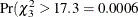 ). Varying the conditional probabilities by treatment improved the model fit significantly.
Output 39.1.4: Fit Statistics and Parameter Estimates in Binomial Cluster Model
| Parameter Estimates for Binomial Cluster Model | |||||||
|---|---|---|---|---|---|---|---|
| Component | Effect | pht | tcpo | Estimate | Standard Error |
z Value | Pr > |z| |
| 1 | Intercept | 1.8213 | 0.5889 | 3.09 | 0.0020 | ||
| 1 | pht | 0 | -1.4962 | 0.6630 | -2.26 | 0.0240 | |
| 1 | pht | 60 | 0 | . | . | . | |
| 1 | tcpo | 0 | -3.1828 | 1.1261 | -2.83 | 0.0047 | |
| 1 | tcpo | 100 | 0 | . | . | . | |
| 1 | pht*tcpo | 0 | 0 | 3.3736 | 1.1953 | 2.82 | 0.0048 |
| 1 | pht*tcpo | 0 | 100 | 0 | . | . | . |
| 1 | pht*tcpo | 60 | 0 | 0 | . | . | . |
| 1 | pht*tcpo | 60 | 100 | 0 | . | . | . |
| Parameter Estimates for Mixing Probabilities | |||||||
|---|---|---|---|---|---|---|---|
| Component | Effect | pht | tcpo | Estimate | Standard Error |
z Value | Pr > |z| |
| 1 | Intercept | -0.7394 | 0.5395 | -1.37 | 0.1705 | ||
| 1 | pht | 0 | 0.4351 | 0.6203 | 0.70 | 0.4830 | |
| 1 | pht | 60 | 0 | . | . | . | |
| 1 | tcpo | 0 | -0.5342 | 0.5893 | -0.91 | 0.3646 | |
| 1 | tcpo | 100 | 0 | . | . | . | |
| 1 | pht*tcpo | 0 | 0 | 1.4055 | 0.7080 | 1.99 | 0.0471 |
| 1 | pht*tcpo | 0 | 100 | 0 | . | . | . |
| 1 | pht*tcpo | 60 | 0 | 0 | . | . | . |
| 1 | pht*tcpo | 60 | 100 | 0 | . | . | . |
Table 39.12 computes the conditional probabilities in the four treatment groups. Recall that the previous model estimated a constant
clustering probability of 0.5831.
Table 39.12: Estimates of Clustering Probabilities
|
PHT |
TCPO |
|
|
|---|---|---|---|
|
0 |
0 |
1.8213 – 1.4962 – 3.1828 + 3.3736 = 0.5159 |
0.6262 |
|
60 |
0 |
1.8213 – 3.1828 = –1.3615 |
0.2040 |
|
0 |
100 |
1.8213 – 1.4962 = 0.3251 |
0.5806 |
|
60 |
100 |
1.8213 |
0.8607 |

The presence of phenytoin alone reduces the probability of response clustering within the litter. The presence of trichloropropene oxide alone does not have a strong effect on the clustering. The simultaneous presence of both agents substantially increases the probability of clustering.
The following statements fit the binomial cluster model in the parameterization of Morel and Neerchal (1997).
proc fmm data=ossi;
   model y/m = x1-x3 / dist=binomcluster;
   probmodel   x1-x3;
run;
The model fit is the same as in the previous model (compare the "Fit Statistics" tables in Output 39.1.5 and Output 39.1.4). The parameter estimates change due to the reparameterization of the treatment effects and match the results in Table III of Morel and Neerchal (1997).
Output 39.1.5: Fit Statistics and Estimates (Morel and Neerchal Parameterization)
The following sets of statements fit the binomial and beta-binomial models, respectively, as single-component mixtures in the parameterization akin to the first binomial cluster model. Note that the model effects that affect the underlying Bernoulli success probabilities are specified in the MODEL statement, in contrast to the binomial cluster model.
proc fmm data=ossi;
   model y/m = x1-x3 / dist=binomial;
run;
proc fmm data=ossi;
   model y/m = x1-x3 / dist=betabinomial;
run;
The Pearson statistic for the beta-binomial model (Output 39.1.6) indicates a much better fit compared to the single-component binomial model (Output 39.1.7). This is not surprising because these data are obviously overdispersed relative to a binomial model because the Bernoulli outcomes are not independent. The difference between the binomial cluster and the beta-binomial model lies in the mechanism by which the correlations are induced:
-
a mixing mechanism in the beta-binomial model that leads to a common shared random effect among all offspring in a cluster
-
a mixture specification in the binomial cluster model that divides the offspring in a litter into identical and independent responders
Output 39.1.6: Fit Statistics in Binomial Model
Output 39.1.7: Fit Statistics in Beta-Binomial Model