The FMM Procedure

Modeling Zero-Inflation: Is It Better to Fish Poorly or Not to Have Fished at All?
The following example shows how you can use PROC FMM to model data that contain more zero values than expected.
Many count data show an excess of zeros relative to the frequency of zeros expected under a reference model. An excess of zeros leads to overdispersion because the process is more variable than a standard count data model. Different mechanisms can lead to excess zeros. For example, suppose that the data are generated from two processes with different distribution functions—one process generates the zero counts, and the other process generates nonzero counts. In the vernacular of Cameron and Trivedi (1998), such a model is called a hurdle model. With a certain probability—the probability of a nonzero count—a hurdle is crossed, and events are being generated. Hurdle models are useful, for example, to model the number of doctor visits per year. Once the decision to see a doctor has been made—the hurdle has been overcome—a certain number of visits follow.
Hurdle models are closely related to zero-inflated models. Both can be expressed as two-component mixtures in which one component has a degenerate distribution at zero and the other component is a count model. In a hurdle model, the count model follows a zero-truncated distribution. In a zero-inflated model, the count model has a nonzero probability of generating zeros. Formally, a zero-inflated model can be written as
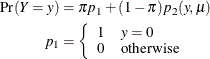
where  is a standard count model with mean
  and support
  .
.
The following data illustrates the use of a zero-inflated model. In a survey of park attendees, randomly selected individuals were asked about the number of fish they caught in the last six months. Along with that count, the gender and age of each sampled individual was recorded. The following DATA step displays the data for the analysis:
data catch;
   input gender $ age count @@;
   datalines;
  F   54  18   M   37   0   F   48  12   M   27   0
  M   55   0   M   32   0   F   49  12   F   45  11
  M   39   0   F   34   1   F   50   0   M   52   4
  M   33   0   M   32   0   F   23   1   F   17   0
  F   44   5   M   44   0   F   26   0   F   30   0
  F   38   0   F   38   0   F   52  18   M   23   1
  F   23   0   M   32   0   F   33   3   M   26   0
  F   46   8   M   45   5   M   51  10   F   48   5
  F   31   2   F   25   1   M   22   0   M   41   0
  M   19   0   M   23   0   M   31   1   M   17   0
  F   21   0   F   44   7   M   28   0   M   47   3
  M   23   0   F   29   3   F   24   0   M   34   1
  F   19   0   F   35   2   M   39   0   M   43   6
;
At first glance, the prevalence of zeros in the DATA set is apparent. Many park attendees did not catch any fish. These zero counts are made up of two populations: attendees who do not fish and attendees who fish poorly. A zero-inflation mechanism thus appears reasonable for this application because a zero count can be produced by two separate distributions.
The following statements fit a standard Poisson regression model to these data. A common intercept is assumed for men and women, and the regression slope varies with gender.
proc fmm data=catch;
   class gender;
   model count = gender*age / dist=Poisson;
run;
Figure 39.7 displays information about the model and data set. The "Model Information" table conveys that the model is a single-component
Poisson model (a Poisson GLM) and that parameters are estimated by maximum likelihood. There are two levels in the CLASS
variable gender, with females preceding males.
Figure 39.7: Model Information and Class Levels in Poisson Regression
The "Fit Statistics" and "Parameter Estimates" tables from the maximum likelihood estimation of the Poisson GLM are shown in Figure 39.8. If the model is not overdispersed, the Pearson statistic should roughly equal the number of observations in the data set minus the number of parameters. With n=52, there is evidence of overdispersion in these data.
Figure 39.8: Fit Results in Poisson Regression
Suppose that the cause of overdispersion is zero-inflation of the count data. The following statements fit a zero-inflated Poisson model.
proc fmm data=catch;
   class gender;
   model count = gender*age / dist=Poisson ;
   model       +            / dist=Constant;
run;
There are two MODEL
statements, one for each component of the mixture. Because the distributions are different for the components, you cannot
specify the mixture model with a single MODEL
statement. The first MODEL
statement identifies the response variable for the model (count) and defines a Poisson model with intercept and gender-specific slopes. The second MODEL
statement uses the continuation operator ("+") and adds a model with a degenerate distribution by using DIST=
CONSTANT. Because the mass of the constant is placed by default at zero, the second MODEL
statement adds a zero-inflation component to the model. It is sufficient to specify the response variable in one of the MODEL
statements; you use the "=" sign in that statement to separate the response variable from the model effects.
Figure 39.9 displays the "Model Information" and "Optimization Information" tables for this run of the FMM procedure. The model is now identified as a zero-inflated Poisson (ZIP) model with two components, and the parameters continue to be estimated by maximum likelihood. The "Optimization Information" table shows that there are four parameters in the optimization (compared to three parameters in the Poisson GLM model). The four parameters correspond to three parameters in the mean function (intercept and two gender-specific slopes) and the mixing probability.
Figure 39.9: Model and Optimization Information in the ZIP Model
Results from fitting the ZIP model by maximum likelihood are shown in Figure 39.10. The –2 log likelihood and the information criteria suggest a much-improved fit over the single-component Poisson model (compare Figure 39.10 to Figure 39.8). The Pearson statistic is reduced by factor 2 compared to the Poisson model and suggests a better fit than the standard Poisson model.
Figure 39.10: Maximum Likelihood Results for the ZIP model
The number of effective parameters and components shown in Figure 39.8 equals the values from Figure 39.9. This is not always the case because components can collapse (for example, when the mixing probability approaches zero or when two components have identical parameter estimates). In this example, both components and all four parameters are identifiable. The Poisson regression and the zero process mix, with a probability of approximately 0.6972 attributed to the Poisson component.
The FMM procedure enables you to fit some mixture models by Bayesian techniques. The following statements add the BAYES statement to the previous PROC FMM statements:
proc fmm data=catch seed=12345;
   class gender;
   model count = gender*age / dist=Poisson;
   model       +            / dist=constant;
   performance cpucount=2;
   bayes;
run;
The "Model Information" table indicates that the model parameters are estimated by Markov chain Monte Carlo techniques, and it displays the random number seed (Figure 39.11). This is useful if you did not specify a seed to identify the seed value that reproduces the current analysis. The "Bayes Information" table provides basic information about the Monte Carlo sampling scheme. The sampling method uses a data augmentation scheme to impute component membership and then the Gamerman (1997) algorithm to sample the component-specific parameters. The 2,000 burn-in samples are followed by 10,000 Monte Carlo samples without thinning.
Figure 39.11: Model, Bayes, and Prior Information in the ZIP Model
The "Prior Distributions" table identifies the prior distributions, their parameters for the sampled quantities, and their initial values. The prior distribution of parameters associated with model effects is a normal distribution with mean 0 and variance 1,000. The prior distribution for the mixing probability is a Dirichlet(1,1), which is identical to a uniform distribution (Figure 39.11). Because the second mixture component is a degeneracy at zero with no associated parameters, it does not appear in the "Prior Distributions" table in Figure 39.11. Figure 39.12 displays descriptive statistics about the 10,000 posterior samples. Recall from Figure 39.10 that the maximum likelihood estimates were –3.5215, 0.1216, 0.1056, and 0.6972, respectively. With this choice of prior, the means of the posterior samples are generally close to the MLEs in this example. The "Posterior Intervals" table displays 95% intervals of equal-tail probability and 95% intervals of highest posterior density (HPD) intervals.
Figure 39.12: Posterior Summaries and Intervals in the ZIP Model
| Posterior Summaries | ||||||||
|---|---|---|---|---|---|---|---|---|
| Component | Effect | gender | N | Mean | Standard Deviation |
Percentiles | ||
| 25 | 50 | 75 | ||||||
| 1 | Intercept | 10000 | -3.5524 | 0.6509 | -3.9922 | -3.5359 | -3.0875 | |
| 1 | age*gender | F | 10000 | 0.1220 | 0.0136 | 0.1124 | 0.1218 | 0.1314 |
| 1 | age*gender | M | 10000 | 0.1058 | 0.0140 | 0.0961 | 0.1055 | 0.1153 |
| 1 | Probability | 10000 | 0.6938 | 0.0945 | 0.6293 | 0.6978 | 0.7605 | |
You can generate trace plots for the posterior parameter estimates by enabling ODS Graphics:
ods graphics on;
ods select TADPanel;
proc fmm data=catch seed=12345;
   class gender;
   model count = gender*age / dist=Poisson;
   model       +            / dist=constant;
   performance cpucount=2;
   bayes;
run;
ods graphics off;
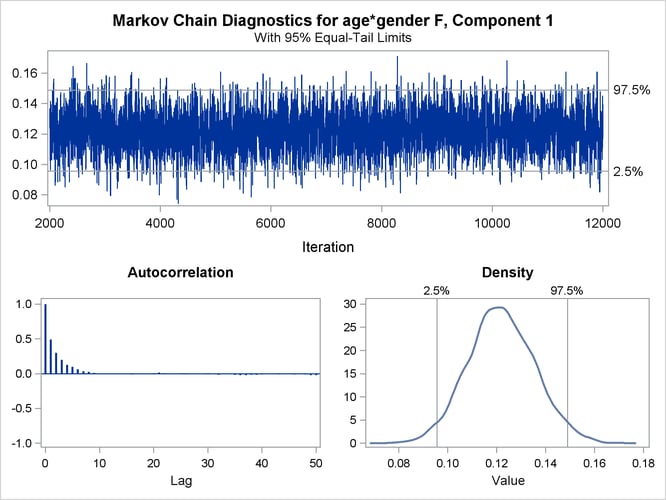
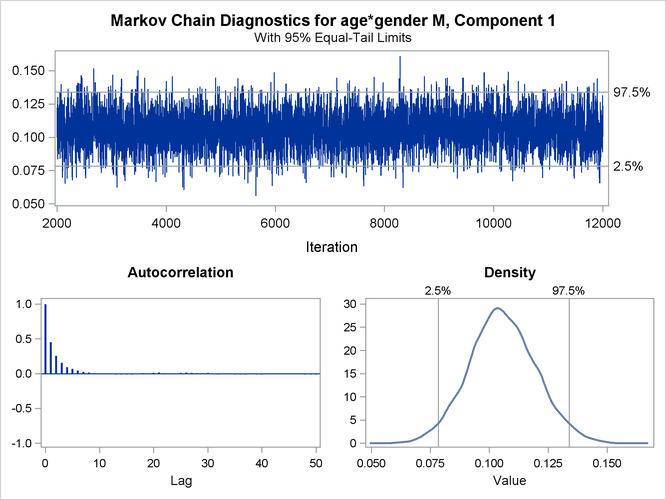
A separate trace panel is produced for each sampled parameter, and the panels for the gender-specific slopes are shown in Figure 39.13. There is good mixing in the chains: the modest autocorrelation that diminishes after about 10 successive samples. By default, the FMM procedure transfers the credible intervals for each parameter from the "Posterior Intervals" table to the trace plot and the density plot in the trace panel.
Figure 39.13: Trace Panels for Gender-Specific Slopes