The FMM Procedure

This example with a mixture of normal and Weibull distributions illustrates the benefits of specifying starting values for some of the components.

The data for this example were generously provided by Dr. Luciano A. Gonzalez of the Lethbridge Research Centre of Agriculture and Agri-Food Canada and his collaborator, Dr. Bert Tolkamp, from the Scottish Agricultural College.

The outcome variable of interest is the logarithm of a time interval between consecutive visits by cattle to feeders. The intervals fall into three categories:

Modeling such time interval data is important to understand the feeding behavior and biology of the animals and to derive other biological parameters such as the probability of an animal to stop eating after it has consumed a certain amount of a given food. Because there are three distinct biological categories, data of this nature are frequently modeled as three-component mixtures. The point at which the second and third components cross over is used to separate feeding events into meals.

The original data set comprises 141,414 observations of log feeding intervals. For the purpose of presentation in this document, where space is limited, the data have been rounded to precision 0.05 and grouped by frequency. The following DATA step displays the modified data used in this example. A comparison with the raw data and the results obtained in a full analysis of the original data show that the grouping does not alter the presentation or conclusions in a way that matters for the purpose of this example.

data cattle;
   input LogInt Count @@;
   datalines;
 0.70   195  1.10   233  1.40   355  1.60   563
 1.80   822  1.95   926  2.10  1018  2.20  1712
 2.30  3190  2.40  2212  2.50  1692  2.55  1558
 2.65  1622  2.70  1637  2.75  1568  2.85  1599
 2.90  1575  2.95  1526  3.00  1537  3.05  1561
 3.10  1555  3.15  1427  3.20  2852  3.25  1396
 3.30  1343  3.35  2473  3.40  1310  3.45  2453
 3.50  1168  3.55  2300  3.60  2174  3.65  2050
 3.70  1926  3.75  1849  3.80  1687  3.85  2416
 3.90  1449  3.95  2095  4.00  1278  4.05  1864
 4.10  1672  4.15  2104  4.20  1443  4.25  1341
 4.30  1685  4.35  1445  4.40  1369  4.45  1284
 4.50  1523  4.55  1367  4.60  1027  4.65  1491
 4.70  1057  4.75  1155  4.80  1095  4.85  1019
 4.90  1158  4.95  1088  5.00  1075  5.05   912
 5.10  1073  5.15   803  5.20   924  5.25   916
 5.30   784  5.35   751  5.40   766  5.45   833
 5.50   748  5.55   725  5.60   674  5.65   690
 5.70   659  5.75   695  5.80   529  5.85   639
 5.90   580  5.95   557  6.00   524  6.05   473
 6.10   538  6.15   444  6.20   456  6.25   453
 6.30   374  6.35   406  6.40   409  6.45   371
 6.50   320  6.55   334  6.60   353  6.65   305
 6.70   302  6.75   301  6.80   263  6.85   218
 6.90   255  6.95   240  7.00   219  7.05   202
 7.10   192  7.15   180  7.20   162  7.25   126
 7.30   148  7.35   173  7.40   142  7.45   163
 7.50   152  7.55   149  7.60   139  7.65   161
 7.70   174  7.75   179  7.80   188  7.85   239
 7.90   225  7.95   213  8.00   235  8.05   256
 8.10   272  8.15   290  8.20   320  8.25   355
 8.30   307  8.35   311  8.40   317  8.45   335
 8.50   369  8.55   365  8.60   365  8.65   396
 8.70   419  8.75   467  8.80   468  8.85   515
 8.90   558  8.95   623  9.00   712  9.05   716
 9.10   829  9.15   803  9.20   834  9.25   856
 9.30   838  9.35   842  9.40   826  9.45   834
 9.50   798  9.55   801  9.60   780  9.65   849
 9.70   779  9.75   737  9.80   683  9.85   686
 9.90   626  9.95   582 10.00   522 10.05   450
10.10   443 10.15   375 10.20   342 10.25   285
10.30   254 10.35   231 10.40   195 10.45   186
10.50   143 10.55   100 10.60    73 10.65    49
10.70    28 10.75    36 10.80    16 10.85     9
10.90     5 10.95     6 11.00     4 11.05     1
11.15     1 11.25     4 11.30     2 11.35     5
11.40     4 11.45     3 11.50     1
;

If you scan the columns for the Count variable in the DATA step, the prevalence of values between 2 and 5 units of LogInt is apparent, as is a long right tail. To explore these data graphically, the following statements produce a histogram of the data and a kernel density estimate of the density of the LogInt variable.

ods graphics on;
proc kde data=cattle;
   univar LogInt / bwm=4;
   freq count;
run;

Output 39.2.1: Histogram and Kernel Density for LogInt

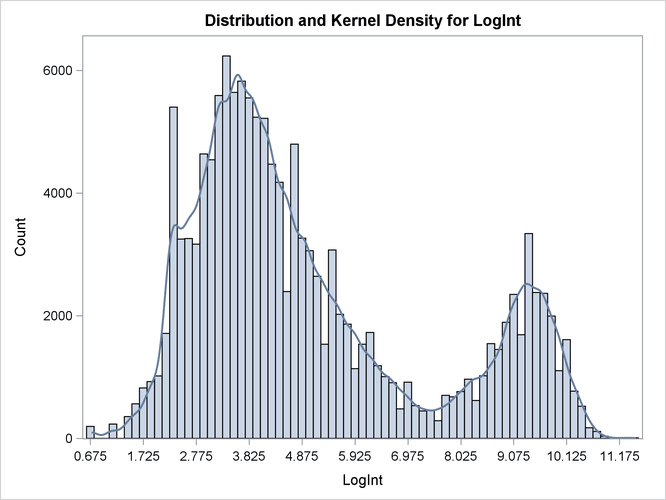
Two modes are clearly visible in Output 39.2.1. Given the biological background, one would expect that three components contribute to the mixture. The histogram would suggest either a two-component mixture with modes near 4 and 9, or a three-component mixture with modes near 3, 5, and 9.

Following Dr. Gonzalez’ suggestion, the process is modeled as a three-component mixture of two normal distributions and a Weibull distribution. The Weibull distribution is chosen because it can have long left and right tails and it is popular in modeling data that relate to time intervals.

proc fmm data=cattle gconv=0;
   model LogInt = / dist=normal k=2 parms(3 1, 5 1);
   model        + / dist=weibull;
   freq count;
run;

The GCONV= convergence criterion is turned off in this PROC FMM run to avoid the early stoppage of the iterations when the relative gradient changes little between iterations. Turning the criterion off usually ensures that convergence is achieved with a small absolute gradient of the objective function. The PARMS option in the first MODEL statement provides starting values for the means and variances for the parameters of the normal distributions. The means for the two components are started at and , respectively. Specifying starting values is generally not necessary. However, the choice of starting values can play an important role in modeling finite mixture models; the importance of the choice of starting values in this example is discussed further below.

The "Model Information" table shows that the model is a three-component mixture and that the FMM procedure considers the estimation of a density to be the purpose of modeling. The procedure draws this conclusion from the absence of effects in the MODEL statements. There are 187 observations in the data set, but these actually represent 141,414 measurements (Output 39.2.2).

There are eight parameters in the optimization: the means and variances of the two normal distributions, the and parameter of the Weibull distribution, and the two mixing probabilities (Output 39.2.3). At the converged solution, the –2 log likelihood is 563,153 and all parameters and components are effective—that is, the model is not overspecified in the sense that components have collapsed during the model fitting. The Pearson statistic is close to the number of observations in the data set, indicating a good fit.

Output 39.2.4 displays the parameter estimates for the three models and for the mixing probabilities. The order in which the "Parameter Estimates" tables appear in the output corresponds to the order in which the MODEL statements were specified.

The estimated means of the two normal components are 3.3415 and 4.8940, respectively. Note that the means are displayed here as Intercept. The inverse linked estimate is not produced because the default link for the normal distribution is the identity link; hence the Estimate column represents the means of the component distributions. The parameter estimates in the Weibull model are , , and 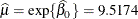. In the Weibull distribution, the parameter does not estimate the mean of the distribution, the maximum likelihood estimate of the distribution’s mean is .

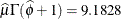The estimated mixing probabilities are , , and . In other words, the estimated distribution of log feeding intervals is a 45:35:20 mixture of an 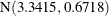, a , and a distribution.

You can obtain a graphical display of the observed and estimated distribution of these data by enabling ODS Graphics. The PLOTS option in the PROC FMM statement modifies the default density plot by adding the densities of the mixture components:

ods select DensityPlot;
proc fmm data=cattle gconv=0;
   model LogInt = / dist=normal k=2 parms(3 1, 5 1);
   model        + / dist=weibull;
   freq count;
run;

Output 39.2.5: Observed and Estimated Densities in the Three-Component Model

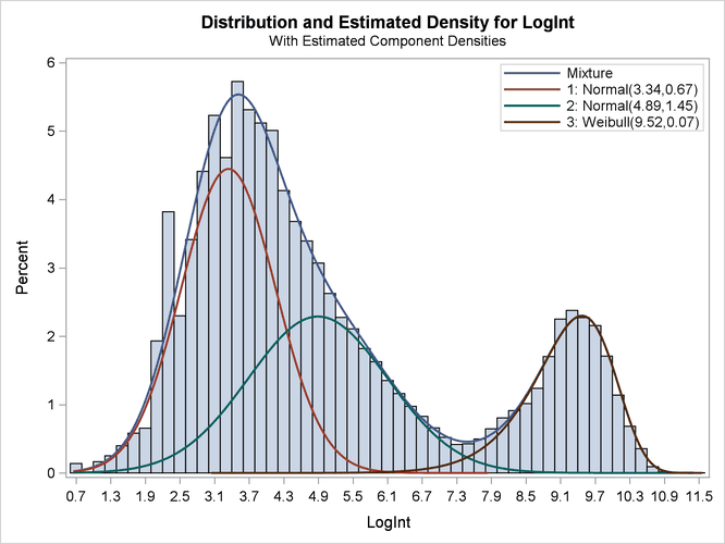
The estimated mixture density matches the histogram of the observed data closely (Output 39.2.5). The component densities are displayed in such a way that, at each point in the support of the LogInt variable, their sum combines to the overall mixture density. The three components in the mixtures are well separated.

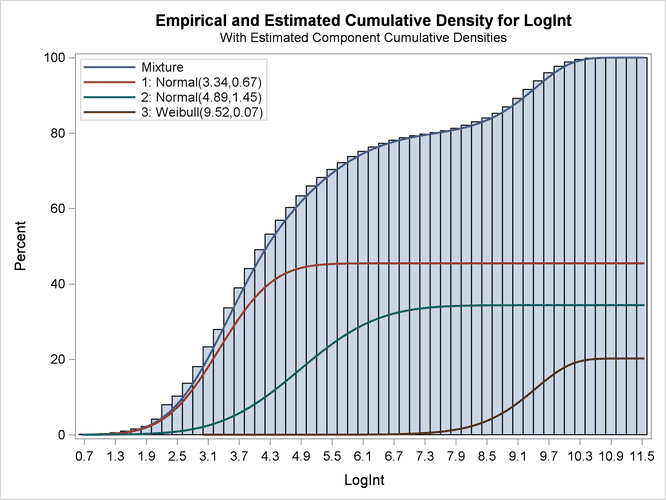
The excellent quality of the fit is even more evident when the distributions are displayed cumulatively by adding the CUMULATIVE option in the DENSITY option (Output 39.2.6):

ods select DensityPlot;
proc fmm data=cattle plot=density(cumulative) gconv=0;
   model LogInt = / dist=normal k=2 parms(3 1, 5 1);
   model        + / dist=weibull;
   freq count;
run;

The component cumulative distribution functions are again scaled so that their sum produces the overall mixture cumulative distribution function. Because of this scaling, the percentage reached at the maximum value of LogInt corresponds to the mixing probabilities in Output 39.2.4.

Output 39.2.6: Observed and Estimated Cumulative Densities in the Three-Component Model

The importance of starting values for the parameter estimates was mentioned previously. Suppose that different starting values are selected for the three components (for example, the default starting values).

proc fmm data=cattle gconv=0;
   model LogInt = / dist=normal k=2;
   model        + / dist=weibull;
   freq count;
run;
ods graphics off;

The fit statistics and parameter estimates from this run are displayed in Output 39.2.7, and the density plot is shown in Output 39.2.8.

All components are active; no collapsing of components occurred. However, a closer look at the "Parameter Estimates" tables in Output 39.2.7 shows an important difference from the tables in Output 39.2.4. The means of the two normal distributions are now 4.9106 and 9.2883. Previously, the means were 3.3415 and 4.8940. The "position" of the Weibull distribution has moved from right to left, and the third component is now modeled by a symmetric normal distribution (Output 39.2.8). The mixture probabilities have also changed—in particular, for the first and third component.

Output 39.2.8: Three-Component Model with Default Starting Values

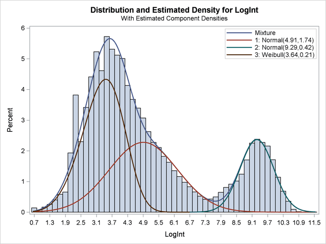
Such switching is not uncommon in mixture modeling. As judged by the information criteria, the model in which the Weibull distribution is the component with the smallest mean does not fit the data as well as the first model in which the specification of the starting values guided the optimization towards placing the normal distributions first. The converged solution found in the last FMM run represents a local minimum of the log-likelihood surface. There are other local minima—for example, when components are removed from the model, which is tantamount to estimating the associated mixture probabilities as zero.