The FMM Procedure

Mixture Modeling for Binomial Overdispersion: "Student," Pearson, Beer, and Yeast
The following example demonstrates how you can model a complicated, two-component binomial mixture distribution, either with maximum likelihood or with Bayesian methods, with a few simple PROC FMM statements.
William Sealy Gosset, a chemist at the Arthur Guinness Son and Company brewery in Dublin, joined the statistical laboratory of Karl Pearson in 1906–1907 to study statistics. At first Gosset—who published all but one paper under the pseudonym "Student" because his employer forbade publications by employees after a co-worker had disclosed trade secrets—worked on the Poisson limit to the binomial distribution, using haemacytometer yeast cell counts. Gosset’s interest in studying small-sample (and limit) problems was motivated by the small sample sizes he typically saw in his work at the brewery.
Subsequently, Gosset’s yeast count data have been examined and revisited by many authors. In 1915, Karl Pearson undertook his own examination and realized that the variability in "Student’s" data exceeded that consistent with a Poisson distribution. Pearson (1915) bemoans the fact that if this were so, "it is certainly most unfortunate that such material should have been selected to illustrate Poisson’s limit to the binomial."
Using a count of Gosset’s yeast cell counts on the 400 squares of a haemacytometer (Table 39.1), Pearson argues that a mixture process would explain the heterogeneity (beyond the Poisson).
Table 39.1: "Student’s" Yeast Cell Counts
|
Number of Cells |
0 |
1 |
2 |
3 |
4 |
5 |
|---|---|---|---|---|---|---|
|
Frequency |
213 |
128 |
37 |
18 |
3 |
1 |
Pearson fits various models to these data, chief among them a mixture of two binomial series
![\[ \nu _1 (p_1 + q_1)^\theta + \nu _2 (p_2 + q_2)^\theta \]](images/statug_fmm0013.png)
where  is real-valued and thus the binomial series expands to
![\[ (p + q)^\theta = \sum _{k=0}^{\infty } \frac{\Gamma (\theta +1)}{\Gamma (k+1)\Gamma (\theta -k+1)} \, p^ k \, q^{\theta -k} \]](images/statug_fmm0015.png)
Pearson’s fitted model has  ,
,  ,
,  (corresponding to a mixing proportion of
  ), and estimated success probabilities in the binomial components of 0.1017 and 0.4514, respectively. The success probabilities
indicate that although the data have about a 90% chance of coming from a distribution with small success probability of about
0.1, there is a 10% chance of coming from a distribution with a much larger success probability of about 0.45.
), and estimated success probabilities in the binomial components of 0.1017 and 0.4514, respectively. The success probabilities
indicate that although the data have about a 90% chance of coming from a distribution with small success probability of about
0.1, there is a 10% chance of coming from a distribution with a much larger success probability of about 0.45.
If is an integer, the binomial series is the cumulative mass function of a binomial random variable. The value of suggests that a suitable model for these data could also be constructed as a two-component mixture of binomial random variables
as follows:
![\[ f(y) = \pi \, \mr{binomial}(5,\mu _1) + (1-\pi )\, \mr{binomial}(5,\mu _2) \]](images/statug_fmm0020.png)
The binomial sample size n=5 is suggested by Pearson’s estimate of  and the fact that the largest cell count in Table 39.1 is 5.
The following DATA step creates a SAS data set from the data in Table 39.1.
data yeast;
   input count f;
   n = 5;
   datalines;
   0     213
   1     128
   2      37
   3      18
   4       3
   5       1
;
The two-component binomial model is fit with the FMM procedure with the following statements:
proc fmm data=yeast;
   model count/n =  / k=2;
   freq f;
run;
Because the events/trials syntax is used in the MODEL statement, PROC FMM defaults to the binomial distribution. The K= 2 option specifies that the number of components is fixed and known to be two. The FREQ statement indicates that the data are grouped; for example, the first observation represents 213 squares on the haemacytometer where no yeast cells were found.
The "Model Information" and "Number of Observations" tables in Figure 39.1 convey that the fitted model is a two-component homogeneous binomial mixture with a logit link function. The mixture is homogeneous because there are no model effects in the MODEL statement and because both component distributions belong to the same distributional family. By default, PROC FMM estimates the model parameters by maximum likelihood.
Although only six observations are read from the data set, the data represent 400 observations (squares on the haemacytometer). Because a constant binomial sample size of 5 is assumed, the data represent 273 successes (finding a yeast cell) out of 2,000 Bernoulli trials.
Figure 39.1: Model Information for Yeast Cell Model
The estimated intercepts (on the logit scale) for the two binomial means are –2.2316 and –0.2974, respectively. These values correspond to binomial success probabilities of 0.09695 and 0.4262, respectively (Figure 39.2). The two components mix with probabilities 0.8799 and 1–0.8799 = 0.1201. These values are generally close to the values found by Pearson (1915) using infinite binomial series instead of binomial mass functions.
Figure 39.2: Maximum Likelihood Estimates
To obtain fitted values and other observationwise statistics under the stipulated two-component model, you can add the OUTPUT statement to the previous PROC FMM run. The following statements request componentwise predicted values and the posterior probabilities:
proc fmm data=yeast;
   model count/n =  / k=2;
   freq f;
   output out=fmmout pred(components) posterior;
run;
data fmmout;
   set fmmout;
   PredCount_1 = post_1 * f;
   PredCount_2 = post_2 * f;
run;
proc print data=fmmout;
run;
The DATA step following the PROC FMM step computes the predicted cell counts in each component (Figure 39.3). The predicted means in the components, 0.48476 and 2.13099, are close to the values determined by Pearson (0.4983 and 2.2118), as are the predicted cell counts.
Figure 39.3: Predicted Cell Counts
| Obs | count | f | n | Pred_1 | Pred_2 | Post_1 | Post_2 | PredCount_1 | PredCount_2 |
|---|---|---|---|---|---|---|---|---|---|
| 1 | 0 | 213 | 5 | 0.096951 | 0.42620 | 0.98606 | 0.01394 | 210.030 | 2.9698 |
| 2 | 1 | 128 | 5 | 0.096951 | 0.42620 | 0.91089 | 0.08911 | 116.594 | 11.4058 |
| 3 | 2 | 37 | 5 | 0.096951 | 0.42620 | 0.59638 | 0.40362 | 22.066 | 14.9341 |
| 4 | 3 | 18 | 5 | 0.096951 | 0.42620 | 0.17598 | 0.82402 | 3.168 | 14.8323 |
| 5 | 4 | 3 | 5 | 0.096951 | 0.42620 | 0.02994 | 0.97006 | 0.090 | 2.9102 |
| 6 | 5 | 1 | 5 | 0.096951 | 0.42620 | 0.00444 | 0.99556 | 0.004 | 0.9956 |
Gosset, who was interested in small-sample statistical problems, investigated the use of prior knowledge in mathematical-statistical analysis—for example, deriving the sampling distribution of the correlation coefficient after having assumed a uniform prior distribution for the coefficient in the population (Aldrich 1997). Pearson also was not opposed to using prior information, especially uniform priors that reflect "equal distribution of ignorance." Fisher, on the other hand, would not have any of it: the best estimator in his opinion is obtained by a criterion that is absolutely independent of prior assumptions about probabilities of particular values. He objected to the insinuation that his derivations in the work on the correlation were deduced from Bayes theorem (Fisher 1921).
The preceding analysis of the yeast cell count data uses maximum likelihood methods that are free of prior assumptions. The following analysis takes instead a Bayesian approach, assuming a beta prior distribution for the binomial success probabilities and a uniform prior distribution for the mixing probabilities. The changes from the previous FMM run are the addition of the ODS GRAPHICS, PERFORMANCE , and BAYES statements and the SEED= 12345 option.
ods graphics on;
proc fmm data=yeast seed=12345;
   model count/n = / k=2;
   freq f;
   performance cpucount=2;
   bayes;
run;
ods graphics off;
With ODS Graphics enabled, PROC FMM produces diagnostic trace plots for the posterior samples. Bayesian analyses are sensitive to the random number seed and thread count; the SEED= and CPUCOUNT= options ensure consistent results for the purposes of this example. The SEED= 12345 option in the PROC FMM statement determines the random number seed for the random number generator used in the analysis. The CPUCOUNT= 2 option in the PERFORMANCE statement sets the number of available processors to two. The BAYES statement requests a Bayesian analysis.
The "Bayes Information" table in Figure 39.4 provides basic information about the Markov chain Monte Carlo sampler. Because the model is a homogeneous mixture, the FMM
procedure applies an efficient conjugate sampling algorithm with a posterior sample size of 10,000 samples after a burn-in
size of 2,000 samples. The "Prior Distributions" table displays the prior distribution for each parameter along with its mean
and variance and the initial value in the chain. Notice that in this situation all three prior distributions reduce to a uniform
distribution on  .
.
Figure 39.4: Basic Information about MCMC Sampler
| Bayes Information | |
|---|---|
| Sampling Algorithm | Conjugate |
| Data Augmentation | Latent Variable |
| Initial Values of Chain | Data Based |
| Burn-In Size | 2000 |
| MC Sample Size | 10000 |
| MC Thinning | 1 |
| Parameters in Sampling | 3 |
| Mean Function Parameters | 2 |
| Scale Parameters | 0 |
| Mixing Prob Parameters | 1 |
| Number of Threads | 2 |
The FMM procedure produces a log note for this model, indicating that the sampled quantities are not the linear predictors on the logit scale, but are the actual population parameters (on the data scale):
NOTE: Bayesian results for this model (no regressor variables,
      non-identity link) are displayed on the data scale, not the
      linked scale. You can obtain results on the linked (=linear)
      scale by requesting a Metropolis-Hastings sampling algorithm.
The trace panel for the success probability in the first binomial component is shown in Figure 39.5. Note that the first component in this Bayesian analysis corresponds to the second component in the MLE analysis. The plots in this panel can be used to diagnose the convergence of the Markov chain. If the chain has not converged, inferences cannot be made based on quantities derived from the chain. You generally look for the following:
-
a smooth unimodal distribution of the posterior estimates in the density plot displayed on the lower right
-
good mixing of the posterior samples in the trace plot at the top of the panel (good mixing is indicated when the trace traverses the support of the distribution and appears to have reached a stationary distribution)
Figure 39.5: Trace Panel for Success Probability in First Component
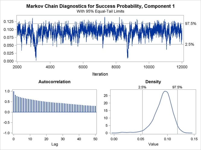
The autocorrelation plot in Figure 39.5 shows fairly high and sustained autocorrelation among the posterior estimates. While this is generally not a problem, you can affect the degree of autocorrelation among the posterior estimates by running a longer chain and thinning the posterior estimates; see the NMC= and THIN= options in the BAYES statement.
Both the trace plot and the density plot in Figure 39.5 are indications of successful convergence.
Figure 39.6 reports selected results that summarize the 10,000 posterior samples. The arithmetic means of the success probabilities in the two components are 0.3884 and 0.0905, respectively. The posterior mean of the mixing probability is 0.1771. These values are similar to the maximum likelihood parameter estimates in Figure 39.2 (after swapping components).
Figure 39.6: Summaries for Posterior Estimates
Note that the standard errors in Figure 39.2 are not comparable to those in Figure 39.6, because the standard errors for the MLEs are expressed on the logit scale and the Bayesian estimates are expressed on the data scale. You can add the METROPOLIS option in the BAYES statement to sample the quantities on the logit scale.
The "Posterior Intervals" table in Figure 39.6 displays 95% credible intervals (equal-tail intervals and intervals of highest posterior density). It can be concluded that the component with the higher success probability contributes less than 40% to the process.