The MIXED Procedure

Example 58.7 Influence in Heterogeneous Variance Model
In this example from Snedecor and Cochran (1976, p. 256), a one-way classification model with heterogeneous variances is fit. The data, shown in the following DATA step, represent amounts of different types of fat absorbed by batches of doughnuts during cooking, measured in grams.
data absorb;
  input FatType Absorbed @@;
  datalines;
 1 164  1 172  1 168  1 177  1 156  1 195
 2 178  2 191  2 197  2 182  2 185  2 177
 3 175  3 193  3 178  3 171  3 163  3 176
 4 155  4 166  4 149  4 164  4 170  4 168
;
The statistical model for these data can be written as
 |
 |
|||
 |
 |
|||
 |
 |
|||
 |
 |
where  is the amount of fat absorbed by the
  th batch of the
  th fat type, and
  denotes the fat-type effects. A quick glance at the data suggests that observations 6, 9, 14, and 21 might be influential on the analysis, because these are extreme observations for the respective fat types.
The following SAS statements fit this model and request influence diagnostics for the fixed effects and covariance parameters. ODS Graphics is used to create plots of the influence diagnostics in addition to the tabular output. The ESTIMATES suboption requests plots of "leave-one-out" estimates for the fixed effects and group variances.
ods graphics on;

proc mixed data=absorb asycov;
   class FatType;
   model Absorbed = FatType / s
                    influence(iter=10 estimates);
   repeated / group=FatType;
   ods output Influence=inf;
run;

ods graphics off;
The "Influence" table is output to the SAS data set inf so that parameter estimates can be printed subsequently. Results from this analysis are shown in Output 58.7.1.
| Model Information | |
|---|---|
| Data Set | WORK.ABSORB |
| Dependent Variable | Absorbed |
| Covariance Structure | Variance Components |
| Group Effect | FatType |
| Estimation Method | REML |
| Residual Variance Method | None |
| Fixed Effects SE Method | Model-Based |
| Degrees of Freedom Method | Between-Within |
| Covariance Parameter Estimates | ||
|---|---|---|
| Cov Parm | Group | Estimate |
| Residual | FatType 1 | 178.00 |
| Residual | FatType 2 | 60.4000 |
| Residual | FatType 3 | 97.6000 |
| Residual | FatType 4 | 67.6000 |
| Solution for Fixed Effects | ||||||
|---|---|---|---|---|---|---|
| Effect | FatType | Estimate | Standard Error | DF | t Value | Pr > |t| |
| Intercept | 162.00 | 3.3566 | 20 | 48.26 | <.0001 | |
| FatType | 1 | 10.0000 | 6.3979 | 20 | 1.56 | 0.1337 |
| FatType | 2 | 23.0000 | 4.6188 | 20 | 4.98 | <.0001 |
| FatType | 3 | 14.0000 | 5.2472 | 20 | 2.67 | 0.0148 |
| FatType | 4 | 0 | . | . | . | . |
The fixed-effects solutions correspond to estimates of the following parameters:
 |
 |
|||
 |
 |
|||
 |
 |
|||
 |
 |
|||
 |
 |
You can easily verify that these estimates are simple functions of the arithmetic means  in the groups. For example,
  ,
,  , and so forth. The covariance parameter estimates are the sample variances in the groups and are uncorrelated.
The variances in the four groups are shown in the "Covariance Parameter Estimates" table (Output 58.7.1). The estimated variance in the first group is two to three times larger than the variance in the other groups.
| Asymptotic Covariance Matrix of Estimates | |||||
|---|---|---|---|---|---|
| Row | Cov Parm | CovP1 | CovP2 | CovP3 | CovP4 |
| 1 | Residual | 12674 | |||
| 2 | Residual | 1459.26 | |||
| 3 | Residual | 3810.30 | |||
| 4 | Residual | 1827.90 | |||
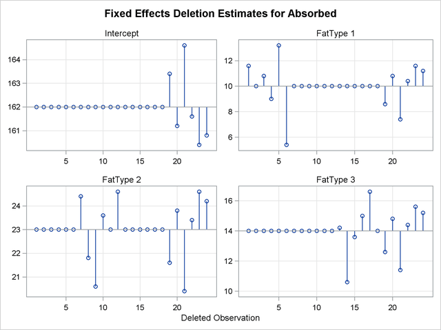
In groups where the residual variance estimate is large, the precision of the estimate is also small (Output 58.7.2).
The following statements print the "leave-one-out" estimates for fixed effects and covariance parameters that were written to the inf data set with the ESTIMATES suboption (Output 58.7.3):
proc print data=inf label;
   var parm1-parm5 covp1-covp4;
run;
| Obs | Intercept | FatType 1 | FatType 2 | FatType 3 | FatType 4 | Residual FatType 1 | Residual FatType 2 | Residual FatType 3 | Residual FatType 4 |
|---|---|---|---|---|---|---|---|---|---|
| 1 | 162.00 | 11.600 | 23.000 | 14.000 | 0 | 203.30 | 60.400 | 97.60 | 67.600 |
| 2 | 162.00 | 10.000 | 23.000 | 14.000 | 0 | 222.47 | 60.400 | 97.60 | 67.600 |
| 3 | 162.00 | 10.800 | 23.000 | 14.000 | 0 | 217.68 | 60.400 | 97.60 | 67.600 |
| 4 | 162.00 | 9.000 | 23.000 | 14.000 | 0 | 214.99 | 60.400 | 97.60 | 67.600 |
| 5 | 162.00 | 13.200 | 23.000 | 14.000 | 0 | 145.70 | 60.400 | 97.60 | 67.600 |
| 6 | 162.00 | 5.400 | 23.000 | 14.000 | 0 | 63.80 | 60.400 | 97.60 | 67.600 |
| 7 | 162.00 | 10.000 | 24.400 | 14.000 | 0 | 178.00 | 60.795 | 97.60 | 67.600 |
| 8 | 162.00 | 10.000 | 21.800 | 14.000 | 0 | 178.00 | 64.691 | 97.60 | 67.600 |
| 9 | 162.00 | 10.000 | 20.600 | 14.000 | 0 | 178.00 | 32.296 | 97.60 | 67.600 |
| 10 | 162.00 | 10.000 | 23.600 | 14.000 | 0 | 178.00 | 72.797 | 97.60 | 67.600 |
| 11 | 162.00 | 10.000 | 23.000 | 14.000 | 0 | 178.00 | 75.490 | 97.60 | 67.600 |
| 12 | 162.00 | 10.000 | 24.600 | 14.000 | 0 | 178.00 | 56.285 | 97.60 | 67.600 |
| 13 | 162.00 | 10.000 | 23.000 | 14.200 | 0 | 178.00 | 60.400 | 121.68 | 67.600 |
| 14 | 162.00 | 10.000 | 23.000 | 10.600 | 0 | 178.00 | 60.400 | 35.30 | 67.600 |
| 15 | 162.00 | 10.000 | 23.000 | 13.600 | 0 | 178.00 | 60.400 | 120.79 | 67.600 |
| 16 | 162.00 | 10.000 | 23.000 | 15.000 | 0 | 178.00 | 60.400 | 114.50 | 67.600 |
| 17 | 162.00 | 10.000 | 23.000 | 16.600 | 0 | 178.00 | 60.400 | 71.30 | 67.600 |
| 18 | 162.00 | 10.000 | 23.000 | 14.000 | 0 | 178.00 | 60.400 | 121.98 | 67.600 |
| 19 | 163.40 | 8.600 | 21.600 | 12.600 | 0 | 178.00 | 60.400 | 97.60 | 69.799 |
| 20 | 161.20 | 10.800 | 23.800 | 14.800 | 0 | 178.00 | 60.400 | 97.60 | 79.698 |
| 21 | 164.60 | 7.400 | 20.400 | 11.400 | 0 | 178.00 | 60.400 | 97.60 | 33.800 |
| 22 | 161.60 | 10.400 | 23.400 | 14.400 | 0 | 178.00 | 60.400 | 97.60 | 83.292 |
| 23 | 160.40 | 11.600 | 24.600 | 15.600 | 0 | 178.00 | 60.400 | 97.60 | 65.299 |
| 24 | 160.80 | 11.200 | 24.200 | 15.200 | 0 | 178.00 | 60.400 | 97.60 | 73.677 |
The graphical displays in Output 58.7.4 and Output 58.7.5 are created when ODS Graphics is enabled. For general information about ODS Graphics, see Chapter 21, Statistical Graphics Using ODS. For specific information about the graphics available in the MIXED procedure, see the section ODS Graphics.
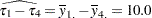
The estimate of the intercept is affected only when observations from the last group are removed. The estimate of the "FatType 1" effect reacts to removal of observations in the first and last group (Output 58.7.4).
While observations can affect one or more fixed-effects solutions in this model, they can affect only one covariance parameter, the variance in their group (Output 58.7.5). Observations 6, 9, 14, and 21, which are extreme in their group, reduce the group variance considerably.
Diagnostics related to residuals and predicted values are printed with the following statements:
proc print data=inf label;
   var observed predicted residual pressres
       student Rstudent;
run;
| Obs | Observed Value |
Predicted Mean | Residual | PRESS Residual | Internally Studentized Residual |
Externally Studentized Residual |
|---|---|---|---|---|---|---|
| 1 | 164 | 172.0 | -8.000 | -9.600 | -0.6569 | -0.6146 |
| 2 | 172 | 172.0 | 0.000 | 0.000 | 0.0000 | 0.0000 |
| 3 | 168 | 172.0 | -4.000 | -4.800 | -0.3284 | -0.2970 |
| 4 | 177 | 172.0 | 5.000 | 6.000 | 0.4105 | 0.3736 |
| 5 | 156 | 172.0 | -16.000 | -19.200 | -1.3137 | -1.4521 |
| 6 | 195 | 172.0 | 23.000 | 27.600 | 1.8885 | 3.1544 |
| 7 | 178 | 185.0 | -7.000 | -8.400 | -0.9867 | -0.9835 |
| 8 | 191 | 185.0 | 6.000 | 7.200 | 0.8457 | 0.8172 |
| 9 | 197 | 185.0 | 12.000 | 14.400 | 1.6914 | 2.3131 |
| 10 | 182 | 185.0 | -3.000 | -3.600 | -0.4229 | -0.3852 |
| 11 | 185 | 185.0 | 0.000 | -0.000 | 0.0000 | 0.0000 |
| 12 | 177 | 185.0 | -8.000 | -9.600 | -1.1276 | -1.1681 |
| 13 | 175 | 176.0 | -1.000 | -1.200 | -0.1109 | -0.0993 |
| 14 | 193 | 176.0 | 17.000 | 20.400 | 1.8850 | 3.1344 |
| 15 | 178 | 176.0 | 2.000 | 2.400 | 0.2218 | 0.1993 |
| 16 | 171 | 176.0 | -5.000 | -6.000 | -0.5544 | -0.5119 |
| 17 | 163 | 176.0 | -13.000 | -15.600 | -1.4415 | -1.6865 |
| 18 | 176 | 176.0 | 0.000 | 0.000 | 0.0000 | 0.0000 |
| 19 | 155 | 162.0 | -7.000 | -8.400 | -0.9326 | -0.9178 |
| 20 | 166 | 162.0 | 4.000 | 4.800 | 0.5329 | 0.4908 |
| 21 | 149 | 162.0 | -13.000 | -15.600 | -1.7321 | -2.4495 |
| 22 | 164 | 162.0 | 2.000 | 2.400 | 0.2665 | 0.2401 |
| 23 | 170 | 162.0 | 8.000 | 9.600 | 1.0659 | 1.0845 |
| 24 | 168 | 162.0 | 6.000 | 7.200 | 0.7994 | 0.7657 |
Observations 6, 9, 14, and 21 have large studentized residuals (Output 58.7.6). That the externally studentized residuals are much larger than the internally studentized residuals for these observations indicates that the variance estimate in the group shrinks when the observation is removed. Also important to note is that comparisons based on raw residuals in models with heterogeneous variance can be misleading. Observation 5, for example, has a larger residual but a smaller studentized residual than observation 21. The variance for the first fat type is much larger than the variance in the fourth group. A "large" residual is more "surprising" in the groups with small variance.
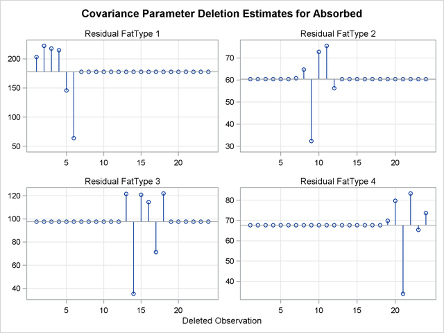
A measure of the overall influence on the analysis is the (restricted) likelihood distance, shown in Output 58.7.7. Observations 6, 9, 14, and 21 clearly displace the REML solution more than any other observations.
The following statements list the restricted likelihood distance and various diagnostics related to the fixed-effects estimates (Output 58.7.8):
proc print data=inf label;
   var leverage observed CookD DFFITS CovRatio RLD;
run;
| Obs | Leverage | Observed Value |
Cook's D | DFFITS | COVRATIO | Restr. Likelihood Distance |
|---|---|---|---|---|---|---|
| 1 | 0.167 | 164 | 0.02157 | -0.27487 | 1.3706 | 0.1178 |
| 2 | 0.167 | 172 | 0.00000 | -0.00000 | 1.4998 | 0.1156 |
| 3 | 0.167 | 168 | 0.00539 | -0.13282 | 1.4675 | 0.1124 |
| 4 | 0.167 | 177 | 0.00843 | 0.16706 | 1.4494 | 0.1117 |
| 5 | 0.167 | 156 | 0.08629 | -0.64938 | 0.9822 | 0.5290 |
| 6 | 0.167 | 195 | 0.17831 | 1.41069 | 0.4301 | 5.8101 |
| 7 | 0.167 | 178 | 0.04868 | -0.43982 | 1.2078 | 0.1935 |
| 8 | 0.167 | 191 | 0.03576 | 0.36546 | 1.2853 | 0.1451 |
| 9 | 0.167 | 197 | 0.14305 | 1.03446 | 0.6416 | 2.2909 |
| 10 | 0.167 | 182 | 0.00894 | -0.17225 | 1.4463 | 0.1116 |
| 11 | 0.167 | 185 | 0.00000 | -0.00000 | 1.4998 | 0.1156 |
| 12 | 0.167 | 177 | 0.06358 | -0.52239 | 1.1183 | 0.2856 |
| 13 | 0.167 | 175 | 0.00061 | -0.04441 | 1.4961 | 0.1151 |
| 14 | 0.167 | 193 | 0.17766 | 1.40175 | 0.4340 | 5.7044 |
| 15 | 0.167 | 178 | 0.00246 | 0.08915 | 1.4851 | 0.1139 |
| 16 | 0.167 | 171 | 0.01537 | -0.22892 | 1.4078 | 0.1129 |
| 17 | 0.167 | 163 | 0.10389 | -0.75423 | 0.8766 | 0.8433 |
| 18 | 0.167 | 176 | 0.00000 | 0.00000 | 1.4998 | 0.1156 |
| 19 | 0.167 | 155 | 0.04349 | -0.41047 | 1.2390 | 0.1710 |
| 20 | 0.167 | 166 | 0.01420 | 0.21950 | 1.4148 | 0.1124 |
| 21 | 0.167 | 149 | 0.15000 | -1.09545 | 0.6000 | 2.7343 |
| 22 | 0.167 | 164 | 0.00355 | 0.10736 | 1.4786 | 0.1133 |
| 23 | 0.167 | 170 | 0.05680 | 0.48500 | 1.1592 | 0.2383 |
| 24 | 0.167 | 168 | 0.03195 | 0.34245 | 1.3079 | 0.1353 |
In this example, observations with large likelihood distances also have large values for Cook’s  and values of CovRatio far less than one (Output 58.7.8). The latter indicates that the fixed effects are estimated more precisely when these observations are removed from the analysis.
The following statements print the values of the statistic and the CovRatio for the covariance parameters:
proc print data=inf label;
   var iter CookDCP CovRatioCP;
run;
The same conclusions as for the fixed-effects estimates hold for the covariance parameter estimates. Observations 6, 9, 14, and 21 change the estimates and their precision considerably (Output 58.7.9, Output 58.7.10). All iterative updates converged within at most four iterations.
| Obs | Iterations | Cook's D CovParms | COVRATIO CovParms |
|---|---|---|---|
| 1 | 3 | 0.05050 | 1.6306 |
| 2 | 3 | 0.15603 | 1.9520 |
| 3 | 3 | 0.12426 | 1.8692 |
| 4 | 3 | 0.10796 | 1.8233 |
| 5 | 4 | 0.08232 | 0.8375 |
| 6 | 4 | 1.02909 | 0.1606 |
| 7 | 1 | 0.00011 | 1.2662 |
| 8 | 2 | 0.01262 | 1.4335 |
| 9 | 3 | 0.54126 | 0.3573 |
| 10 | 3 | 0.10531 | 1.8156 |
| 11 | 3 | 0.15603 | 1.9520 |
| 12 | 2 | 0.01160 | 1.0849 |
| 13 | 3 | 0.15223 | 1.9425 |
| 14 | 4 | 1.01865 | 0.1635 |
| 15 | 3 | 0.14111 | 1.9141 |
| 16 | 3 | 0.07494 | 1.7203 |
| 17 | 3 | 0.18154 | 0.6671 |
| 18 | 3 | 0.15603 | 1.9520 |
| 19 | 2 | 0.00265 | 1.3326 |
| 20 | 3 | 0.08008 | 1.7374 |
| 21 | 1 | 0.62500 | 0.3125 |
| 22 | 3 | 0.13472 | 1.8974 |
| 23 | 2 | 0.00290 | 1.1663 |
| 24 | 2 | 0.02020 | 1.4839 |
Output 58.7.10 displays the standard panel of influence diagnostics that is obtained when influence analysis is iterative. The Cook’s and CovRatio statistics are displayed for each deletion set for both fixed-effects and covariance parameter estimates. This provides a convenient summary of the impact on the analysis for each deletion set, since Cook’s statistic measures impact on the estimates and the CovRatio statistic measures impact on the precision of the estimates.
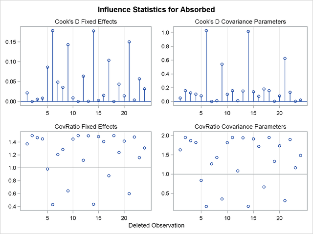
Observations 6, 9, 14, and 21 have considerable impact on estimates and precision of fixed effects and covariance parameters. This is not necessarily the case. Observations can be influential on only some aspects of the analysis, as shown in the next example.