The MIXED Procedure

Intercept

By default, all models automatically include a column of 1s in to estimate a fixed-effect intercept parameter . You can use the NOINT option in the MODEL statement to suppress this intercept. The NOINT option is useful when you are specifying a classification effect in the MODEL statement and you want the parameter estimate to be in terms of the mean response for each level of that effect, rather than in terms of a deviation from an overall mean.

By contrast, the intercept is not included by default in . To obtain a column of 1s in , you must specify in the RANDOM statement either the INTERCEPT effect or some effect that has only one level.

Regression Effects

Numeric variables, or polynomial terms involving them, can be included in the model as regression effects (covariates). The actual values of such terms are included as columns of the model matrices and . You can use the bar operator with a regression effect to generate polynomial effects. For instance, X|X|X expands to X X*X X*X*X, a cubic model.

Main Effects

If a classification variable has m levels, PROC MIXED generates m columns in the model matrix for its main effect. Each column is an indicator variable for a given level. The order of the columns is the sort order of the values of their levels and can be controlled with the ORDER= option in the PROC MIXED statement. Table 58.16 is an example.

Typically, there are more columns for these effects than there are degrees of freedom for them. In other words, PROC MIXED uses an overparameterized model.

Interaction Effects

Often a model includes interaction (crossed) effects. With an interaction, PROC MIXED first reorders the terms to correspond to the order of the variables in the CLASS statement. Thus, B*A becomes A*B if A precedes B in the CLASS statement. Then, PROC MIXED generates columns for all combinations of levels that occur in the data. The order of the columns is such that the rightmost variables in the cross index faster than the leftmost variables (Table 58.17). Empty columns (that would contain all 0s) are not generated for , but they are for .

In the preceding matrix, main-effects columns are not linearly independent of crossed-effects columns; in fact, the column space for the crossed effects contains the space of the main effect.

When your model contains many interaction effects, you might be able to code them more parsimoniously by using the bar operator (|). The bar operator generates all possible interaction effects. For example, A|B|C expands to A B A*B C A*C B*C A*B*C. To eliminate higher-order interaction effects, use the at sign (@) in conjunction with the bar operator. For instance, A|B|C|D @2 expands to A B A*B C A*C B*C D A*D B*D C*D.

Nested Effects

Nested effects are generated in the same manner as crossed effects. Hence, the design columns generated by the following two statements are the same (but the ordering of the columns is different):

model Y=A B(A);

model Y=A A*B;

The nesting operator in PROC MIXED is more a notational convenience than an operation distinct from crossing. Nested effects are typically characterized by the property that the nested variables never appear as main effects. The order of the variables within nesting parentheses is made to correspond to the order of these variables in the CLASS statement. The order of the columns is such that variables outside the parentheses index faster than those inside the parentheses, and the rightmost nested variables index faster than the leftmost variables (Table 58.18).

Note that nested effects are often distinguished from interaction effects by the implied randomization structure of the design. That is, they usually indicate random effects within a fixed-effects framework. The fact that random effects can be modeled directly in the RANDOM statement might make the specification of nested effects in the MODEL statement unnecessary.

Continuous-Nesting-Class Effects

When a continuous variable nests with a classification variable, the design columns are constructed by multiplying the continuous values into the design columns for the class effect (Table 58.19).

This model estimates a separate slope for X within each level of A.

Continuous-by-Class Effects

Continuous-by-class effects generate the same design columns as continuous-nesting-class effects. The two models are made different by the presence of the continuous variable as a regressor by itself, as well as a contributor to a compound effect. Table 58.20 shows an example.

You can use continuous-by-class effects to test for homogeneity of slopes.

General Effects

An example that combines all the effects is X1*X2*A*B*C (D E). The continuous list comes first, followed by the crossed list, followed by the nested list in parentheses. You should be aware of the sequencing of parameters when you use the CONTRAST or ESTIMATE statement to compute some function of the parameter estimates.

Effects might be renamed by PROC MIXED to correspond to ordering rules. For example, B*A(E D) might be renamed A*B(D E) to satisfy the following:

• Classification variables that occur outside parentheses (crossed effects) are sorted in the order in which they appear in the CLASS statement.

• Variables within parentheses (nested effects) are sorted in the order in which they appear in the CLASS statement.

The sequencing of the parameters generated by an effect can be described by which variables have their levels indexed faster:

• Variables in the crossed list index faster than variables in the nested list.

• Within a crossed or nested list, variables to the right index faster than variables to the left.

For example, suppose a model includes four effects—A, B, C, and D—each having two levels, 1 and 2. Suppose the CLASS statement is as follows:

class A B C D;

Then the order of the parameters for the effect B*A(C D), which is renamed A*B (C D), is

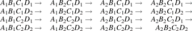Note that first the crossed effects B and A are sorted in the order in which they appear in the CLASS statement so that A precedes B in the parameter list. Then, for each combination of the nested effects in turn, combinations of A and B appear. The B effect moves fastest because it is rightmost in the cross list. Then A moves next fastest, and D moves next fastest. The C effect is the slowest since it is leftmost in the nested list.

When numeric levels are used, levels are sorted by their character format, which might not correspond to their numeric sort sequence (for example, noninteger levels). Therefore, it is advisable to include a desired format for numeric levels or to use the ORDER=INTERNAL option in the PROC MIXED statement to ensure that levels are sorted by their internal values.

Implications of the Non-Full-Rank Parameterization

For models with fixed effects involving classification variables, there are more design columns in constructed than there are degrees of freedom for the effect. Thus, there are linear dependencies among the columns of . In this event, all of the parameters are not estimable; there is an infinite number of solutions to the mixed model equations. PROC MIXED uses a generalized inverse (a -inverse, Pringle and Rayner, 1971) to obtain values for the estimates (Searle 1971). The solution values are not displayed unless you specify the SOLUTION option in the MODEL statement. The solution has the characteristic that estimates are 0 whenever the design column for that parameter is a linear combination of previous columns. With this parameterization, hypothesis tests are constructed to test linear functions of the parameters that are estimable.

Some procedures (such as the CATMOD procedure) reparameterize models to full rank by using restrictions on the parameters. PROC GLM and PROC MIXED do not reparameterize, making the hypotheses that are commonly tested more understandable. See Goodnight (1978) for additional reasons for not reparameterizing.

Missing Level Combinations

PROC MIXED handles missing level combinations of classification variables similarly to the way PROC GLM does. Both procedures delete fixed-effects parameters corresponding to missing levels in order to preserve estimability. However, PROC MIXED does not delete missing level combinations for random-effects parameters because linear combinations of the random-effects parameters are always estimable. These conventions can affect the way you specify your CONTRAST and ESTIMATE coefficients.