The MIXED Procedure

Model Information

The "Model Information" table describes the model, some of the variables it involves, and the method used in fitting it. It also lists the method (profile, factor, parameter, or none) for handling the residual variance in the model. The profile method concentrates the residual variance out of the optimization problem, whereas the parameter method retains it as a parameter in the optimization. The factor method keeps the residual fixed, and none is displayed when a residual variance is not part of the model.

The "Model Information" table also has a row labeled Fixed Effects SE Method. This row describes the method used to compute the approximate standard errors for the fixed-effects parameter estimates and related functions of them. The two possibilities for this row are Model-Based, which is the default method, and Empirical, which results from using the EMPIRICAL option in the PROC MIXED statement.

For ODS purposes, the name of the "Model Information" table is "ModelInfo."

Class Level Information

The "Class Level Information" table lists the levels of every variable specified in the CLASS statement. You should check this information to make sure the data are correct. You can adjust the order of the CLASS variable levels with the ORDER= option in the PROC MIXED statement. For ODS purposes, the name of the "Class Level Information" table is "ClassLevels."

Dimensions

The "Dimensions" table lists the sizes of relevant matrices. This table can be useful in determining CPU time and memory requirements. For ODS purposes, the name of the "Dimensions" table is "Dimensions."

Number of Observations

The "Number of Observations" table shows the number of observations read from the data set and the number of observations used in fitting the model.

Iteration History

The "Iteration History" table describes the optimization of the residual log likelihood or log likelihood. The function to be minimized (the objective function) is for ML and for REML; the column name of the objective function in the "Iteration History" table is "-2 Log Like" for ML and "-2 Res Log Like" for REML. The minimization is performed by using a ridge-stabilized Newton-Raphson algorithm, and the rows of this table describe the iterations that this algorithm takes in order to minimize the objective function.

The Evaluations column of the "Iteration History" table tells how many times the objective function is evaluated during each iteration.

The Criterion column of the "Iteration History" table is, by default, a relative Hessian convergence quantity given by

where is the value of the objective function at iteration k, is the gradient (first derivative) of , and is the Hessian (second derivative) of . If is singular, then PROC MIXED uses the following relative quantity:

To prevent the division by , use the ABSOLUTE option in the PROC MIXED statement. To use a relative function or gradient criterion, use the CONVF or CONVG option, respectively.

The Hessian criterion is considered superior to function and gradient criteria because it measures orthogonality rather than lack of progress (Bates and Watts 1988). Provided the initial estimate is feasible and the maximum number of iterations is not exceeded, the Newton-Raphson algorithm is considered to have converged when the criterion is less than the tolerance specified with the CONVF, CONVG, or CONVH option in the PROC MIXED statement. The default tolerance is 1E8. If convergence is not achieved, PROC MIXED displays the estimates of the parameters at the last iteration.

A convergence criterion that is missing indicates that a boundary constraint has been dropped; it is usually not a cause for concern.

If you specify the ITDETAILS option in the PROC MIXED statement, then the covariance parameter estimates at each iteration are included as additional columns in the "Iteration History" table.

For ODS purposes, the name of the "Iteration History" table is "IterHistory."

Convergence Status

The "Convergence Status" table informs about the status of the iterative estimation process at the end of the Newton-Raphson optimization. It appears as a message in the listing, and this message is repeated in the log. The ODS object "ConvergenceStatus" also contains several nonprinting columns that can be helpful in checking the success of the iterative process, in particular during batch processing or when analyzing BY groups. The Status variable takes on the value 0 for a successful convergence (even if the Hessian matrix might not be positive definite). The values 1 and 2 of the Status variable indicate lack of convergence and infeasible initial parameter values, respectively. The variables pdG and pdH can be used to check whether the and (Hessian) matrices are positive definite.

For models that are not fit iteratively, such as models without random effects or when the NOITER option is in effect, the "Convergence Status" is not produced.

Covariance Parameter Estimates

The "Covariance Parameter Estimates" table contains the estimates of the parameters in and (see the section Estimating Covariance Parameters in the Mixed Model). Their values are labeled in the table along with Subject and Group information if applicable. The estimates are displayed in the Estimate column and are the results of one of the following estimation methods: REML, ML, MIVQUE0, SSCP, Type1, Type2, or Type3.

If you specify the RATIO option in the PROC MIXED statement, the Ratio column is added to the table listing the ratio of each parameter estimate to that of the residual variance.

Specifying the COVTEST option in the PROC MIXED statement produces the "Std Error," "Z Value," and "Pr Z" columns. The "Std Error" column contains the approximate standard errors of the covariance parameter estimates. These are the square roots of the diagonal elements of the observed inverse Fisher information matrix, which equals , where is the Hessian matrix. The matrix consists of the second derivatives of the objective function with respect to the covariance parameters; see Wolfinger, Tobias, and Sall (1994) for formulas. When you use the SCORING= option and PROC MIXED converges without stopping the scoring algorithm, PROC MIXED uses the expected Hessian matrix to compute the covariance matrix instead of the observed Hessian. The observed or expected inverse Fisher information matrix can be viewed as an asymptotic covariance matrix of the estimates.

The "Z Value" column is the estimate divided by its approximate standard error, and the "Pr Z" column is the one- or two-tailed area of the standard Gaussian density outside of the Z-value. The MIXED procedure computes one-sided p-values for the residual variance and for covariance parameters with a lower bound of 0. The procedure computes two-sided p-values otherwise. These statistics constitute Wald tests of the covariance parameters, and they are valid only asymptotically.

Caution: Wald tests can be unreliable in small samples.

For ODS purposes, the name of the "Covariance Parameter Estimates" table is "CovParms."

Fit Statistics

The "Fit Statistics" table provides some statistics about the estimated mixed model. Expressions for the times the log likelihood are provided in the section Estimating Covariance Parameters in the Mixed Model. If the log likelihood is an extremely large number, then PROC MIXED has deemed the estimated matrix to be singular. In this case, all subsequent results should be viewed with caution.

In addition, the "Fit Statistics" table lists three information criteria: AIC, AICC, and BIC, all in smaller-is-better form. Expressions for these criteria are described under the IC option.

For ODS purposes, the name of the "Model Fitting Information" table is "FitStatistics."

Null Model Likelihood Ratio Test

If one covariance model is a submodel of another, you can carry out a likelihood ratio test for the significance of the more general model by computing times the difference between their log likelihoods. Then compare this statistic to the distribution with degrees of freedom equal to the difference in the number of parameters for the two models.

This test is reported in the "Null Model Likelihood Ratio Test" table to determine whether it is necessary to model the covariance structure of the data at all. The "Chi-Square" value is times the log likelihood from the null model minus times the log likelihood from the fitted model, where the null model is the one with only the fixed effects listed in the MODEL statement and . This statistic has an asymptotic distribution with degrees of freedom, where q is the effective number of covariance parameters (those not estimated to be on a boundary constraint). The "Pr > ChiSq" column contains the upper-tail area from this distribution. This p-value can be used to assess the significance of the model fit.

This test is not produced for cases where the null hypothesis lies on the boundary of the parameter space, which is typically for variance component models. This is because the standard asymptotic theory does not apply in this case (Self and Liang 1987, Case 5).

If you specify a PARMS statement, PROC MIXED constructs a likelihood ratio test between the best model from the grid search and the final fitted model and reports the results in the "Parameter Search" table.

For ODS purposes, the name of the "Null Model Likelihood Ratio Test" table is "LRT."

Type 3 Tests of Fixed Effects

The "Type 3 Tests of Fixed Effects" table contains hypothesis tests for the significance of each of the fixed effects—that is, those effects you specify in the MODEL statement. By default, PROC MIXED computes these tests by first constructing a Type 3 matrix (see Chapter 15, The Four Types of Estimable Functions ) for each effect. This matrix is then used to compute the following F statistic:

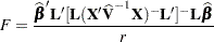where 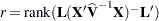. A -value for the test is computed as the tail area beyond this statistic from an F distribution with NDF and DDF degrees of freedom. The numerator degrees of freedom (NDF) are the row rank of , and the denominator degrees of freedom are computed by using one of the methods described under the DDFM= option. Small values of the -value (typically less than 0.05 or 0.01) indicate a significant effect.

You can use the HTYPE= option in the MODEL statement to obtain tables of Type 1 (sequential) tests and Type 2 (adjusted) tests in addition to or instead of the table of Type 3 (partial) tests.

You can use the CHISQ option in the MODEL statement to obtain Wald tests of the fixed effects. These are carried out by using the numerator of the F statistic and comparing it with the distribution with NDF degrees of freedom. It is more liberal than the F test because it effectively assumes infinite denominator degrees of freedom.

For ODS purposes, the names of the "Type 1 Tests of Fixed Effects" through the "Type 3 Tests of Fixed Effects" tables are "Tests1" through "Tests3," respectively.