The MIXED Procedure

| REPEATED Statement |
The REPEATED statement is used to specify the  matrix in the mixed model. Its syntax is different from that of the REPEATED statement in PROC GLM. If no REPEATED statement is specified, is assumed to be equal to
  .
.
For many repeated measures models, no repeated effect is required in the REPEATED statement. Simply use the SUBJECT= option to define the blocks of and the TYPE= option to define their covariance structure. In this case, the repeated measures data must be similarly ordered for each subject, and you must indicate all missing response variables with periods in the input data set unless they all fall at the end of a subject’s repeated response profile. These requirements are necessary in order to inform PROC MIXED of the proper location of the observed repeated responses.
Specifying a repeated effect is useful when you do not want to indicate missing values with periods in the input data set. The repeated effect must contain only classification variables. Make sure that the levels of the repeated effect are different for each observation within a subject; otherwise, PROC MIXED constructs identical rows in corresponding to the observations with the same level. This results in a singular and an infinite likelihood.
Whether you specify a REPEATED effect or not, the rows of for each subject are constructed in the order in which they appear in the input data set.
Table 58.12 summarizes important options in the REPEATED statement. All options are subsequently discussed in alphabetical order.
Option |
Description |
|---|---|
Construction of Covariance Structure |
|
Defines an effect specifying heterogeneity in the R-side covariance structure |
|
Specifies data set with coefficient matrices for TYPE=LIN |
|
Requests that a diagonal matrix be added to |
|
Specifies that only the local effects are weighted |
|
Specifies that only the nonlocal effects are weighted |
|
Identifies the subjects in the R-side model |
|
Specifies the R-side covariance structure |
|
Statistical Output |
|
Produces a table of Hotelling-Lawley-McKeon statistics (McKeon 1974) |
|
Produces a table of Hotelling-Lawley-Pillai-Samson statistics (Pillai and Samson 1959) |
|
Displays blocks of the estimated |
|
Display the Cholesky root (lower) of blocks of the estimated |
|
Displays the inverse Cholesky root (lower) of blocks of the estimated |
|
Displays the correlation matrix corresponding to blocks of the estimated |
|
Displays the inverse of blocks of the estimated |
|
You can specify the following options in the REPEATED statement after a slash (/).
- GROUP=effect
- GRP=effect
-
defines an effect that specifies heterogeneity in the covariance structure of
. All observations that have the same level of the GROUP effect have the same covariance parameters. Each new level of the GROUP effect produces a new set of covariance parameters with the same structure as the original group. You should exercise caution in properly defining the GROUP effect, because strange covariance patterns can result with its misuse. Also, the GROUP effect can greatly increase the number of estimated covariance parameters, which can adversely affect the optimization process. Continuous variables are permitted as arguments to the GROUP= option. PROC MIXED does not sort by the values of the continuous variable; rather, it considers the data to be from a new subject or group whenever the value of the continuous variable changes from the previous observation. Using a continuous variable decreases execution time for models with a large number of subjects or groups and also prevents the production of a large "Class Level Information" table.
- HLM
-
produces a table of Hotelling-Lawley-McKeon statistics (McKeon 1974) for all fixed effects whose levels change across data having the same level of the SUBJECT= effect (the within-subject fixed effects). This option applies only when you specify a REPEATED statement with the TYPE=UN option and no RANDOM statements. For balanced data, this model is equivalent to the multivariate model for repeated measures in PROC GLM.
The Hotelling-Lawley-McKeon statistic has a slightly better
 approximation than the Hotelling-Lawley-Pillai-Samson statistic (see the description of the HLPS option, which follows). Both of the Hotelling-Lawley statistics can perform much better in small samples than the default statistic (Wright 1994).
 Separate tables are produced for Type 1, 2, and 3 tests, according to the ones you select. For ODS purposes, the table names are "HLM1," "HLM2," and "HLM3," respectively.
- HLPS
-
produces a table of Hotelling-Lawley-Pillai-Samson statistics (Pillai and Samson 1959) for all fixed effects whose levels change across data having the same level of the SUBJECT= effect (the within-subject fixed effects). This option applies only when you specify a REPEATED statement with the TYPE=UN option and no RANDOM statements. For balanced data, this model is equivalent to the multivariate model for repeated measures in PROC GLM, and this statistic is the same as the Hotelling-Lawley Trace statistic produced by PROC GLM.
Separate tables are produced for Type 1, 2, and 3 tests, according to the ones you select. For ODS purposes, the table names are "HLPS1," "HLPS2," and "HLPS3," respectively.
- LDATA=SAS-data-set
-
reads the coefficient matrices associated with the TYPE=LIN(number) option. The data set must contain the variables Parm, Row, Col1–Coln or Parm, Row, Col, Value. The Parm variable denotes which of the number coefficient matrices is currently being constructed, and the Row, Col1–Coln, or Row, Col, Value variables specify the matrix values, as they do with the RANDOM statement option GDATA=. Unspecified values of these matrices are set equal to 0.
- LOCAL
- LOCAL=POM(POM-data-set)
-
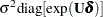
requests that a diagonal matrix be added to
. With just the LOCAL option, this diagonal matrix equals , and  becomes an additional variance parameter that PROC MIXED profiles out of the likelihood provided that you do not specify the NOPROFILE option in the PROC MIXED statement. The LOCAL option is useful if you want to add an observational error to a time series structure (Jones and Boadi-Boateng 1991) or a nugget effect to a spatial structure (Cressie 1993).
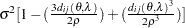
 The LOCAL=EXP(<effects>) option produces exponential local effects, also known as dispersion effects, in a log-linear variance model. These local effects have the form
where
 is the full-rank design matrix corresponding to the effects that you specify and
  are the parameters that PROC MIXED estimates. An intercept is not included in because it is accounted for by
  . PROC MIXED constructs the full-rank in terms of 1s and
  1s for classification effects. Be sure to scale continuous effects in sensibly.
 The LOCAL=POM(POM-data-set) option specifies the power-of-the-mean structure. This structure possesses a variance of the form
 for the
  th observation, where
  is the th row of
  (the design matrix of the fixed effects) and
  is an estimate of the fixed-effects parameters that you specify in POM-data-set.
 The SAS data set specified by POM-data-set contains the numeric variable Estimate (in previous releases, the variable name was required to be EST), and it has at least as many observations as there are fixed-effects parameters. The first
 observations of the Estimate variable in POM-data-set are taken to be the elements of , where is the number of columns of
  . You must order these observations according to the non-full-rank parameterization of the MIXED procedure. One easy way to set up POM-data-set for a corresponding to ordinary least squares is illustrated by the following statements:
 ods output SolutionF=sf; proc mixed; class a; model y = a x / s; run; proc mixed; class a; model y = a x; repeated / local=pom(sf); run;
Note that the generalized least squares estimate of the fixed-effects parameters from the second PROC MIXED step usually is not the same as your specified
. However, you can iterate the POM fitting until the two estimates agree. Continuing from the previous example, the statements for performing one step of this iteration are as follows: ods output SolutionF=sf1; proc mixed; class a; model y = a x / s; repeated / local=pom(sf); run; proc compare brief data=sf compare=sf1; var estimate; run; data sf; set sf1; run;
Unfortunately, this iterative process does not always converge. For further details, refer to the description of pseudo-likelihood in Chapter 3 of Carroll and Ruppert (1988).
- LOCALW
specifies that only the local effects and no others be weighted. By default, all effects are weighted. The LOCALW option is used in connection with the WEIGHT statement and the LOCAL option in the REPEATED statement.
- NONLOCALW
specifies that only the nonlocal effects and no others be weighted. By default, all effects are weighted. The NONLOCALW option is used in connection with the WEIGHT statement and the LOCAL option in the REPEATED statement.
- R<=value-list>
-
requests that blocks of the estimated
matrix be displayed. The first block determined by the SUBJECT= effect is the default displayed block. PROC MIXED displays blanks for value-lists that are 0. The value-list indicates the subjects for which blocks of
are to be displayed. For example, the following statement displays block matrices for the first, third, and fifth persons: repeated / type=cs subject=person r=1,3,5;
See the PARMS statement for the possible forms of value-list. The table name for ODS purposes is "R."
- RC<=value-list>
produces the Cholesky root of blocks of the estimated
matrix. The value-list specification is the same as with the R option. The table name for ODS purposes is "CholR." - RCI<=value-list>
produces the inverse Cholesky root of blocks of the estimated
matrix. The value-list specification is the same as with the R option. The table name for ODS purposes is "InvCholR." - RCORR<=value-list>
produces the correlation matrix corresponding to blocks of the estimated
matrix. The value-list specification is the same as with the R option. The table name for ODS purposes is "RCorr." - RI<=value-list>
produces the inverse of blocks of the estimated
matrix. The value-list specification is the same as with the R option. The table name for ODS purposes is "InvR." - SSCP
-
requests that an unstructured
matrix be estimated from the sum-of-squares-and-crossproducts matrix of the residuals. It applies only when you specify TYPE=UN and have no RANDOM statements. Also, you must have a sufficient number of subjects for the estimate to be positive definite. This option is useful when the size of the blocks of
is large (for example, greater than 10) and you want to use or inspect an unstructured estimate that is much quicker to compute than the default REML estimate. The two estimates will agree for certain balanced data sets when you have a classification fixed effect defined across all time points within a subject. - SUBJECT=effect
- SUB=effect
-
identifies the subjects in your mixed model. Complete independence is assumed across subjects; therefore, the SUBJECT= option produces a block-diagonal structure in
with identical blocks. When the SUBJECT= effect consists entirely of classification variables, the blocks of correspond to observations sharing the same level of that effect. These blocks are sorted according to this effect as well. Continuous variables are permitted as arguments to the SUBJECT= option. PROC MIXED does not sort by the values of the continuous variable; rather, it considers the data to be from a new subject or group whenever the value of the continuous variable changes from the previous observation. Using a continuous variable decreases execution time for models with a large number of subjects or groups and also prevents the production of a large "Class Level Information" table.
If you want to model nonzero covariance among all of the observations in your SAS data set, specify SUBJECT=INTERCEPT to treat the data as if they are all from one subject. However, be aware that in this case PROC MIXED manipulates an
matrix with dimensions equal to the number of observations. If no SUBJECT= effect is specified, then every observation is assumed to be from a different subject and is assumed to be diagonal. For this reason, you usually want to use the SUBJECT= option in the REPEATED statement. - TYPE=covariance-structure
-
specifies the covariance structure of the
matrix. The SUBJECT= option defines the blocks of , and the TYPE= option specifies the structure of these blocks. Valid values for covariance-structure and their descriptions are provided in Table 58.13 and Table 58.14. The default structure is VC. Table 58.13 Covariance Structures Structure
Description
Parms
 th element
 ANTE(1)
Antedependence


AR(1)
Autoregressive(1)
2

ARH(1)
Heterogeneous AR(1)


ARMA(1,1)
ARMA(1,1)
3

CS
Compound symmetry
2

CSH
Heterogeneous CS
FA(
 )
) Factor analytic

FA0(
) No diagonal FA


FA1(
) Equal diagonal FA
HF
Huynh-Feldt

LIN(
) General linear

TOEP
Toeplitz


TOEP(
) Banded Toeplitz

TOEPH
Heterogeneous TOEP

TOEPH(
) Banded hetero TOEP

UN
Unstructured


UN(
) Banded


UNR
Unstructured corrs
UNR(
) Banded correlations
UN@AR(1)
Direct product AR(1)


UN@CS
Direct product CS

UN@UN
Direct product UN


VC
Variance components

and i corresponds to kth effect
In Table 58.13, "Parms" is the number of covariance parameters in the structure,
is the overall dimension of the covariance matrix, and  equals 1 when
  is true and 0 otherwise. For example, 1
 equals 1 when
  and 0 otherwise, and 1
 equals 1 when
  and 0 otherwise. For the TYPE=TOEPH structures,
  , and for the TYPE=UNR structures,
  for all . For the direct product structures, the subscripts "1" and "2" refer to the first and second structure in the direct product, respectively, and
 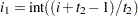 ,
,  ,
,  , and
, and  .
. Table 58.14 Spatial Covariance Structures Structure
Description
Parms
th element SP(EXP)(c-list )
Exponential
2
SP(EXPA)(c-list )
Anisotropic exponential

SP(EXPGA)(
 )
) 2D exponential,
4
geometrically anisotropic
SP(GAU)(c-list )
Gaussian
2
SP(GAUGA)(
) 2D Gaussian,
4
geometrically anisotropic
SP(LIN)(c-list )
Linear
2
SP(LINL)(c-list )
Linear log
2

SP(MATERN)(c-list)
Matérn
3
SP(MATHSW)(c-list)
Matérn
3
(Handcock-Stein-Wallis)
SP(POW)(c-list)
Power
2

SP(POWA)(c-list)
Anisotropic power

SP(SPH)(c-list )
Spherical
2
SP(SPHGA)(
) 2D Spherical,
4
geometrically anisotropic
In Table 58.14, c-list contains the names of the numeric variables used as coordinates of the location of the observation in space, and
 is the Euclidean distance between the ith and jth vectors of these coordinates, which correspond to the ith and jth observations in the input data set. For SP(POWA) and SP(EXPA), c is the number of coordinates, and
  is the absolute distance between the kth coordinate,
  , of the ith and jth observations in the input data set. For the geometrically anisotropic structures SP(EXPGA), SP(GAUGA), and SP(SPHGA), exactly two spatial coordinate variables must be specified as
  and
and  . Geometric anisotropy is corrected by applying a rotation
  and scaling
  to the coordinate system, and
  represents the Euclidean distance between two points in the transformed space. SP(MATERN) and SP(MATHSW) represent covariance structures in a class defined by Matérn (see Matérn 1986, Handcock and Stein 1993, Handcock and Wallis 1994). The function
  is the modified Bessel function of the second kind of (real) order
  ; the parameter
  governs the smoothness of the process (see below for more details).
 Table 58.15 lists some examples of the structures in Table 58.13 and Table 58.14.
Table 58.15 Covariance Structure Examples Description
Structure
Example
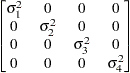
Variance
componentsVC (default)
Compound
symmetryCS
Unstructured
UN
Banded main
diagonalUN(1)
First-order
autoregressiveAR(1)

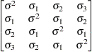
Toeplitz
TOEP
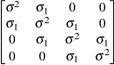
Toeplitz with
two bandsTOEP(2)
Spatial
powerSP(POW)(c)

Heterogeneous
AR(1)ARH(1)
First-order
autoregressive
moving averageARMA(1,1)

Heterogeneous
CSCSH
First-order
factor
analyticFA(1)
Huynh-Feldt
HF
First-order
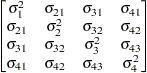
antedependenceANTE(1)

Heterogeneous
ToeplitzTOEPH
Unstructured
correlationsUNR
Direct product
AR(1)UN@AR(1)
The following provides some further information about these covariance structures:
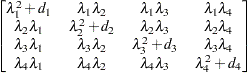
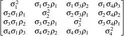
- TYPE=ANTE(1)
-
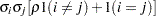
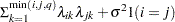
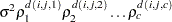
specifies the first-order antedependence structure (see Kenward 1987, Patel 1991, and Macchiavelli and Arnold 1994). In Table 58.13,
 is the th variance parameter, and
  is the
  th autocorrelation parameter satisfying
  .
. - TYPE=AR(1)
-
specifies a first-order autoregressive structure. PROC MIXED imposes the constraint
 for stationarity.
 - TYPE=ARH(1)
-
specifies a heterogeneous first-order autoregressive structure. As with TYPE=AR(1), PROC MIXED imposes the constraint
for stationarity. - TYPE=ARMA(1,1)
-
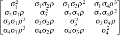
specifies the first-order autoregressive moving-average structure. In Table 58.13,
 is the autoregressive parameter,
  models a moving-average component, and is the residual variance. In the notation of Fuller (1976, p. 68),
  and
and 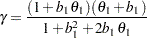
The example in Table 58.15 and
 imply that
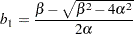
where
 and
and 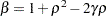 . PROC MIXED imposes the constraints and
  for stationarity, although for some values of and in this region the resulting covariance matrix is not positive definite. When the estimated value of becomes negative, the computed covariance is multiplied by
  to account for the negativity.
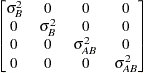
 - TYPE=CS
-
specifies the compound-symmetry structure, which has constant variance and constant covariance.
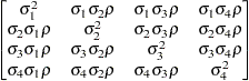
- TYPE=CSH
-
specifies the heterogeneous compound-symmetry structure. This structure has a different variance parameter for each diagonal element, and it uses the square roots of these parameters in the off-diagonal entries. In Table 58.13,
is the th variance parameter, and is the correlation parameter satisfying . - TYPE=FA(q)
-
specifies the factor-analytic structure with q factors (Jennrich and Schluchter 1986). This structure is of the form
 , where
  is a
is a  rectangular matrix and
  is a
is a  diagonal matrix with different parameters. When
  , the elements of in its upper-right corner (that is, the elements in the th row and
  th column for
  ) are set to zero to fix the rotation of the structure.
 - TYPE=FA0(q)
-
is similar to the FA(
) structure except that no diagonal matrix is included. When  —that is, when the number of factors is less than the dimension of the matrix—this structure is nonnegative definite but not of full rank. In this situation, you can use it for approximating an unstructured
  matrix in the RANDOM statement or for combining with the LOCAL option in the REPEATED statement. When
  , you can use this structure to constrain to be nonnegative definite in the RANDOM statement.
 - TYPE=FA1(q)
-
is similar to the TYPE=FA(q) structure except that all of the elements in
are constrained to be equal. This offers a useful and more parsimonious alternative to the full factor-analytic structure. - TYPE=HF
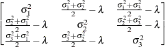
-
specifies the Huynh-Feldt covariance structure (Huynh and Feldt 1970). This structure is similar to the TYPE=CSH structure in that it has the same number of parameters and heterogeneity along the main diagonal. However, it constructs the off-diagonal elements by taking arithmetic rather than geometric means.
You can perform a likelihood ratio test of the Huynh-Feldt conditions by running PROC MIXED twice, once with TYPE=HF and once with TYPE=UN, and then subtracting their respective values of
 times the maximized likelihood.
 If PROC MIXED does not converge under your Huynh-Feldt model, you can specify your own starting values with the PARMS statement. The default MIVQUE(0) starting values can sometimes be poor for this structure. A good choice for starting values is often the parameter estimates corresponding to an initial fit that uses TYPE=CS.
- TYPE=LIN(q)
-
specifies the general linear covariance structure with
parameters. This structure consists of a linear combination of known matrices that are input with the LDATA= option. This structure is very general, and you need to make sure that the variance matrix is positive definite. By default, PROC MIXED sets the initial values of the parameters to 1. You can use the PARMS statement to specify other initial values. - TYPE=SIMPLE
-
is an alias for TYPE=VC.
- TYPE=SP(EXPA)(c-list)
-
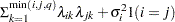
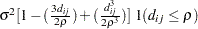
specifies the spatial anisotropic exponential structure, where c-list is a list of variables indicating the coordinates. This structure has
th element equal to 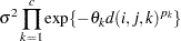
where
 is the number of coordinates and is the absolute distance between the th coordinate (
 ) of the th and th observations in the input data set. There are parameters to be estimated:
  ,
,  (), and .
 You might want to constrain some of the EXPA parameters to known values. For example, suppose you have three coordinate variables C1, C2, and C3 and you want to constrain the powers
to equal 2, as in Sacks et al. (1989). Suppose further that you want to model covariance across the entire input data set and you suspect the and estimates are close to 3, 4, 5, and 1, respectively. Then specify the following statements: repeated / type=sp(expa)(c1 c2 c3) subject=intercept; parms (3) (4) (5) (2) (2) (2) (1) / hold=4,5,6;
- TYPE=SP(EXPGA)(
 )
) - TYPE=SP(GAUGA)()
- TYPE=SP(SPHGA)()
-
specify modifications of the isotropic SP(EXP), SP(SPH), and SP(GAU) covariance structures that allow for geometric anisotropy in two dimensions. The coordinates are specified by the variables c1 and c2.
If the spatial process is geometrically anisotropic in
 , then it is isotropic in the coordinate system
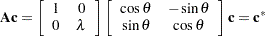
for a properly chosen angle
and scaling factor . Elliptical isocorrelation contours are thereby transformed to spherical contours, adding two parameters to the respective isotropic covariance structures. Euclidean distances (see Table 58.14) are expressed in terms of  .
. The angle
of the clockwise rotation is reported in radians,  . The scaling parameter represents the ratio of the range parameters in the direction of the major and minor axis of the correlation contours. In other words, following a rotation of the coordinate system by angle , isotropy is achieved by compressing or magnifying distances in one coordinate by the factor .
 Fixing
 reduces the models to isotropic ones for any angle of rotation. If the scaling parameter is held constant at 1.0, you should also hold constant the angle of rotation, as in the following statements:
 repeated / type=sp(expga)(gxc gyc) subject=intercept; parms (6) (1.0) (0.0) (1) / hold=2,3;If
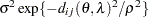
is fixed at any other value than 1.0, the angle of rotation can be estimated. Specifying a starting grid of angles and scaling factors can considerably improve the convergence properties of the optimization algorithm for these models. Only a single random effect with geometrically anisotropic structure is permitted. - TYPE=SP(MATERN)(c-list )
- TYPE=SP(MATHSW)(c-list )
-
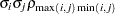
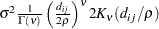
specifies covariance structures in the Matérn class of covariance functions (Matérn 1986). Two observations for the same subject (block of
) that are Euclidean distance apart have covariance 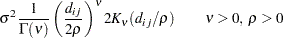
where
 is the modified Bessel function of the second kind of (real) order . The smoothness (continuity) of a stochastic process with covariance function in this class increases with . The Matérn class thus enables data-driven estimation of the smoothness properties. The covariance is identical to the exponential model for
  (TYPE=SP(EXP)(c-list)), while for
  the model advocated by Whittle (1954) results. As
  the model approaches the gaussian covariance structure (TYPE=SP(GAU)(c-list)).
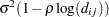
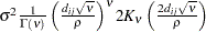
 The MATHSW structure represents the Matérn class in the parameterization of Handcock and Stein (1993) and Handcock and Wallis (1994),
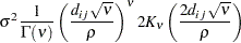
Since computation of the function
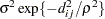
and its derivatives is numerically very intensive, fitting models with Matérn covariance structures can be more time-consuming than with other spatial covariance structures. Good starting values are essential. - TYPE=SP(POW)(c-list)
- TYPE=SP(POWA)(c-list)
-
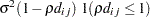
specifies the spatial power structures. When the estimated value of
becomes negative, the computed covariance is multiplied by to account for the negativity. - TYPE=TOEP<(q)>
-
specifies a banded Toeplitz structure. This can be viewed as a moving-average structure with order equal to
 . The TYPE=TOEP option is a full Toeplitz matrix, which can be viewed as an autoregressive structure with order equal to the dimension of the matrix. The specification TYPE=TOEP(1) is the same as
  , where
  is an identity matrix, and it can be useful for specifying the same variance component for several effects.
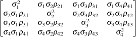
 - TYPE=TOEPH<(q)>
-
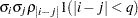
specifies a heterogeneous banded Toeplitz structure. In
Table 58.13, is the th variance parameter and  is the th correlation parameter satisfying
  . If you specify the order parameter q, then PROC MIXED estimates only the first bands of the matrix, setting all higher bands equal to 0. The option TOEPH(1) is equivalent to both the TYPE=UN(1) and TYPE=UNR(1) options.
 - TYPE=UN<(q)>
-
specifies a completely general (unstructured) covariance matrix parameterized directly in terms of variances and covariances. The variances are constrained to be nonnegative, and the covariances are unconstrained. This structure is not constrained to be nonnegative definite in order to avoid nonlinear constraints; however, you can use the TYPE=FA0 structure if you want this constraint to be imposed by a Cholesky factorization. If you specify the order parameter q, then PROC MIXED estimates only the first q bands of the matrix, setting all higher bands equal to 0.
- TYPE=UNR<(q)>
-
specifies a completely general (unstructured) covariance matrix parameterized in terms of variances and correlations. This structure fits the same model as the TYPE=UN(
) option but with a different parameterization. The th variance parameter is . The parameter  is the correlation between the th and th measurements; it satisfies
  . If you specify the order parameter
  , then PROC MIXED estimates only the first q bands of the matrix, setting all higher bands equal to zero.
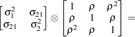
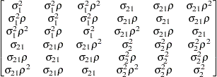
 - TYPE=UN@AR(1)
- TYPE=UN@CS
- TYPE=UN@UN
-
specify direct (Kronecker) product structures designed for multivariate repeated measures (see Galecki 1994). These structures are constructed by taking the Kronecker product of an unstructured matrix (modeling covariance across the multivariate observations) with an additional covariance matrix (modeling covariance across time or another factor). The upper-left value in the second matrix is constrained to equal 1 to identify the model. See the SAS/IML User’s Guide for more details about direct products.
To use these structures in the REPEATED statement, you must specify two distinct REPEATED effects, both of which must be included in the CLASS statement. The first effect indicates the multivariate observations, and the second identifies the levels of time or some additional factor. Note that the input data set must still be constructed in "univariate" format; that is, all dependent observations are still listed observation-wise in one single variable. Although this construction provides for general modeling possibilities, it forces you to construct variables indicating both dimensions of the Kronecker product.
For example, suppose your observed data consist of heights and weights of several children measured over several successive years. Your input data set should then contain variables similar to the following:
Y, all of the heights and weights, with a separate observation for each
Var, indicating whether the measurement is a height or a weight
Year, indicating the year of measurement
Child, indicating the child on which the measurement was taken
Your PROC MIXED statements for a Kronecker AR(1) structure across years would then be as follows:
proc mixed;
   class Var Year Child;
   model Y = Var Year Var*Year;
   repeated Var Year / type=un@ar(1)
                       subject=Child;
run;
You should nearly always want to model different means for the multivariate observations; hence the inclusion of Var in the MODEL statement. The preceding mean model consists of cell means for all combinations of VAR and YEAR.
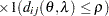
- TYPE=VC
specifies standard variance components and is the default structure for both the RANDOM and REPEATED statements. In the RANDOM statement, a distinct variance component is assigned to each effect. In the REPEATED statement, this structure is usually used only with the GROUP= option to specify a heterogeneous variance model.
Jennrich and Schluchter (1986) provide general information about the use of covariance structures, and Wolfinger (1996) presents details about many of the heterogeneous structures. Modeling with spatial covariance structures is discussed in many sources, for example, Marx and Thompson (1987), Zimmerman and Harville (1991), Cressie (1993), Brownie, Bowman, and Burton (1993), Stroup, Baenziger, and Mulitze (1994), Brownie and Gumpertz (1997), Gotway and Stroup (1997), Chilès and Delfiner (1999), Schabenberger and Gotway (2005), and Littell et al. (2006).