The MIXED Procedure

MODEL Statement

MODEL dependent = <fixed-effects></ options> ;

The MODEL statement names a single dependent variable and the fixed effects, which determine the $\text{[math]}$ matrix of the mixed model (see the section Parameterization of Mixed Models for details). The specification of effects is the same as in the GLM procedure; however, unlike PROC GLM, you do not specify random effects in the MODEL statement. The MODEL statement is required.

An intercept is included in the fixed-effects model by default. If no fixed effects are specified, only this intercept term is fit. The intercept can be removed by using the NOINT option.

Table 58.6 summarizes options in the MODEL statement. These are subsequently discussed in detail in alphabetical order.

Table 58.6 Summary of Important MODEL Statement Options
Option	Description
Model Building
NOINT	Excludes fixed-effect intercept from model
Statistical Computations
ALPHA= $\text{[math]}$	Determines the confidence level ( $\text{[math]}$ ) for fixed effects
ALPHAP= $\text{[math]}$	Determines the confidence level ( $\text{[math]}$ ) for predicted values
CHISQ	Requests chi-square tests
DDF=	Specifies denominator degrees of freedom (list)
DDFM=	Specifies the method for computing denominator degrees of freedom
HTYPE=	Selects the type of hypothesis test
INFLUENCE	Requests influence and case-deletion diagnostics
NOTEST	Suppresses hypothesis tests for the fixed effects
OUTP=	Specifies output data set for predicted values and related quantities
OUTPM=	Specifies output data set for predicted values and related quantities
RESIDUAL	Adds Pearson-type and studentized residuals to output data sets
VCIRY	Adds scaled marginal residual to output data sets
Statistical Output
CL	Displays confidence limits for fixed-effects parameter estimates
CORRB	Displays correlation matrix of fixed-effects parameter estimates
COVB	Displays covariance matrix of fixed-effects parameter estimates
COVBI	Displays inverse covariance matrix of fixed-effects parameter estimates
E, E1, E2, E3	Displays $\text{[math]}$ matrix coefficients
INTERCEPT	Adds a row for the intercept to test tables
SOLUTION	Displays fixed-effects parameter estimates (and scale parameter in GLM models)
Singularity Tolerances
SINGCHOL=	Tunes sensitivity in computing Cholesky roots
SINGRES=	Tunes singularity criterion for residual variance
SINGULAR=	Tunes the sensitivity in sweeping
ZETA=	Tunes the sensitivity in forming Type 3 functions

You can specify the following options in the MODEL statement after a slash (/).

ALPHA=number

requests that a t-type confidence interval be constructed for each of the fixed-effects parameters with confidence level $\text{[math]}$ number. The value of number must be between 0 and 1; the default is 0.05.

ALPHAP=number

requests that a t-type confidence interval be constructed for the predicted values with confidence level $\text{[math]}$ number. The value of number must be between 0 and 1; the default is 0.05.

CHISQ

requests that chi-square tests be performed for all specified effects in addition to the F tests. Type 3 tests are the default; you can produce the Type 1 and Type 2 tests by using the HTYPE= option.

CL

requests that t-type confidence limits be constructed for each of the fixed-effects parameter estimates. The confidence level is 0.95 by default; this can be changed with the ALPHA= option.

CONTAIN

has the same effect as the DDFM=CONTAIN option.

CORRB

produces the approximate correlation matrix of the fixed-effects parameter estimates. For ODS purposes, the name of this table is "CorrB."

COVB

produces the approximate variance-covariance matrix of the fixed-effects parameter estimates $\text{[math]}$ . By default, this matrix equals $\text{[math]}$ and results from sweeping $\text{[math]}$ on all but its last pivot and removing the $\text{[math]}$ border. The EMPIRICAL option in the PROC MIXED statement changes this matrix into "empirical sandwich" form. For ODS purposes, the name of this table is "CovB." If the degrees-of-freedom method of Kenward and Roger (1997) is in effect (DDFM=KENWARDROGER), the COVB matrix changes because the method entails an adjustment of the variance-covariance matrix of the fixed effects by the method proposed by Prasad and Rao (1990) and Harville and Jeske (1992); see also Kackar and Harville (1984).

COVBI

produces the inverse of the approximate variance-covariance matrix of the fixed-effects parameter estimates. For ODS purposes, the name of this table is "InvCovB."

DDF=value-list

enables you to specify your own denominator degrees of freedom for the fixed effects. The value-list specification is a list of numbers or missing values (.) separated by commas. The degrees of freedom should be listed in the order in which the effects appear in the "Tests of Fixed Effects" table. If you want to retain the default degrees of freedom for a particular effect, use a missing value for its location in the list. For example, the following statement assigns 3 denominator degrees of freedom to A and 4.7 to A*B, while those for B remain the same:

model Y = A B A*B / ddf=3,.,4.7;

If you specify DDFM=SATTERTHWAITE or DDFM=KENWARDROGER, the DDF= option has no effect.

DDFM=

DDFM=CONTAIN

DDFM=BETWITHIN

DDFM=RESIDUAL

DDFM=SATTERTHWAITE

DDFM=KENWARDROGER<(FIRSTORDER)>

specifies the method for computing the denominator degrees of freedom for the tests of fixed effects resulting from the MODEL, CONTRAST, ESTIMATE, and LSMEANS statements.

Table 58.7 lists syntax aliases for the degrees-of-freedom methods.

Table 58.7 Aliases for DDFM= Option
DDFM= Option	Alias
BETWITHIN	BW
CONTAIN	CON
KENWARDROGER	KENROG, KR
RESIDUAL	RES
SATTERTHWAITE	SATTERTH, SAT

The DDFM=CONTAIN option invokes the containment method to compute denominator degrees of freedom, and it is the default when you specify a RANDOM statement. The containment method is carried out as follows: Denote the fixed effect in question A, and search the RANDOM effect list for the effects that syntactically contain A. For example, the random effect B(A) contains A, but the random effect C does not, even if it has the same levels as B(A).

Among the random effects that contain A, compute their rank contribution to the ( $\text{[math]}$ ) matrix. The DDF assigned to A is the smallest of these rank contributions. If no effects are found, the DDF for A is set equal to the residual degrees of freedom, $\text{[math]}$ . This choice of DDF matches the tests performed for balanced split-plot designs and should be adequate for moderately unbalanced designs.

Caution: If you have a $\text{[math]}$ matrix with a large number of columns, the overall memory requirements and the computing time after convergence can be substantial for the containment method. If it is too large, you might want to use the DDFM=BETWITHIN option.

The DDFM=BETWITHIN option is the default for REPEATED statement specifications (with no RANDOM statements). It is computed by dividing the residual degrees of freedom into between-subject and within-subject portions. PROC MIXED then checks whether a fixed effect changes within any subject. If so, it assigns within-subject degrees of freedom to the effect; otherwise, it assigns the between-subject degrees of freedom to the effect (see Schluchter and Elashoff 1990). If there are multiple within-subject effects containing classification variables, the within-subject degrees of freedom are partitioned into components corresponding to the subject-by-effect interactions.

One exception to the preceding method is the case where you have specified no RANDOM statements and a REPEATED statement with the TYPE=UN option. In this case, all effects are assigned the between-subject degrees of freedom to provide for better small-sample approximations to the relevant sampling distributions. DDFM=KENWARDROGER might be a better option to try for this case.

The DDFM=RESIDUAL option performs all tests by using the residual degrees of freedom, $\text{[math]}$ , where $\text{[math]}$ is the number of observations.

The DDFM=SATTERTHWAITE option performs a general Satterthwaite approximation for the denominator degrees of freedom, computed as follows. Suppose $\text{[math]}$ is the vector of unknown parameters in $\text{[math]}$ , and suppose $\text{[math]}$ , where $\text{[math]}$ denotes a generalized inverse. Let $\text{[math]}$ and $\text{[math]}$ be the corresponding estimates.

Consider the one-dimensional case, and consider $\text{[math]}$ to be a vector defining an estimable linear combination of $\text{[math]}$ . The Satterthwaite degrees of freedom for the t statistic

$\text{[math]}$

is computed as

$\text{[math]}$

where $\text{[math]}$ is the gradient of $\text{[math]}$ with respect to $\text{[math]}$ , evaluated at $\text{[math]}$ , and $\text{[math]}$ is the asymptotic variance-covariance matrix of $\text{[math]}$ obtained from the second derivative matrix of the likelihood equations.

For the multidimensional case, let $\text{[math]}$ be an estimable contrast matrix and denote the rank of $\text{[math]}$ as $\text{[math]}$ . The Satterthwaite denominator degrees of freedom for the F statistic

$\text{[math]}$

are computed by first performing the spectral decomposition $\text{[math]}$ , where $\text{[math]}$ is an orthogonal matrix of eigenvectors and $\text{[math]}$ is a diagonal matrix of eigenvalues, both of dimension $\text{[math]}$ . Define $\text{[math]}$ to be the $\text{[math]}$ th row of $\text{[math]}$ , and let

$\text{[math]}$

where $\text{[math]}$ is the $\text{[math]}$ th diagonal element of $\text{[math]}$ and $\text{[math]}$ is the gradient of $\text{[math]}$ with respect to $\text{[math]}$ , evaluated at $\text{[math]}$ . Then let

$\text{[math]}$

where the indicator function eliminates terms for which $\text{[math]}$ . The degrees of freedom for $\text{[math]}$ are then computed as

$\text{[math]}$

provided $\text{[math]}$ ; otherwise $\text{[math]}$ is set to zero.

This method is a generalization of the techniques described in Giesbrecht and Burns (1985), McLean and Sanders (1988), and Fai and Cornelius (1996). The method can also include estimated random effects. In this case, append $\text{[math]}$ to $\text{[math]}$ and change $\text{[math]}$ to be the inverse of the coefficient matrix in the mixed model equations. The calculations require extra memory to hold $\text{[math]}$ matrices that are the size of the mixed model equations, where $\text{[math]}$ is the number of covariance parameters. In the notation of Table 58.25, this is approximately $\text{[math]}$ bytes. Extra computing time is also required to process these matrices. The Satterthwaite method implemented here is intended to produce an accurate F approximation; however, the results can differ from those produced by PROC GLM. Also, the small sample properties of this approximation have not been extensively investigated for the various models available with PROC MIXED.

The DDFM=KENWARDROGER option performs the degrees of freedom calculations detailed by Kenward and Roger (1997). This approximation involves inflating the estimated variance-covariance matrix of the fixed and random effects by the method proposed by Prasad and Rao (1990) and Harville and Jeske (1992); see also Kackar and Harville (1984). Satterthwaite-type degrees of freedom are then computed based on this adjustment. By default, the observed information matrix of the covariance parameter estimates is used in the calculations. For covariance structures that have nonzero second derivatives with respect to the covariance parameters, the Kenward-Roger covariance matrix adjustment includes a second-order term. This term can result in standard error shrinkage. Also, the resulting adjusted covariance matrix can then be indefinite and is not invariant under reparameterization. The FIRSTORDER suboption of the DDFM=KENWARDROGER option eliminates the second derivatives from the calculation of the covariance matrix adjustment. For the case of scalar estimable functions, the resulting estimator is referred to as the Prasad-Rao estimator $\text{[math]}$ in Harville and Jeske (1992). The following are examples of covariance structures that generally lead to nonzero second derivatives: TYPE=ANTE(1), TYPE=AR(1), TYPE=ARH(1), TYPE=ARMA(1,1), TYPE=CSH, TYPE=FA, TYPE=FA0( $\text{[math]}$ ), TYPE=TOEPH, TYPE=UNR, and all TYPE=SP() structures.

When the asymptotic variance matrix of the covariance parameters is found to be singular, a generalized inverse is used. Covariance parameters with zero variance then do not contribute to the degrees-of-freedom adjustment for DDFM=SATTERTHWAITE and DDFM=KENWARDROGER, and a message is written to the log.

This method changes output in the following tables (listed in Table 58.22): Contrast, CorrB, CovB, Diffs, Estimates, InvCovB, LSMeans, Slices, SolutionF, SolutionR, Tests1–Tests3. The OUTP= and OUTPM= data sets are also affected.

E

requests that Type 1, Type 2, and Type 3 $\text{[math]}$ matrix coefficients be displayed for all specified effects. For ODS purposes, the name of the table is "Coef."

E1

requests that Type 1 $\text{[math]}$ matrix coefficients be displayed for all specified effects. For ODS purposes, the name of the table is "Coef."

E2

requests that Type 2 $\text{[math]}$ matrix coefficients be displayed for all specified effects. For ODS purposes, the name of the table is "Coef."

E3

requests that Type 3 $\text{[math]}$ matrix coefficients be displayed for all specified effects. For ODS purposes, the name of the table is "Coef."

FULLX

requests that columns of the $\text{[math]}$ matrix that consist entirely of zeros not be eliminated from $\text{[math]}$ ; otherwise, they are eliminated by default. For a column corresponding to a missing cell to be added to $\text{[math]}$ , its particular levels must be present in at least one observation in the analysis data set along with a missing dependent variable. The use of the FULLX option can affect coefficient specifications in the CONTRAST and ESTIMATE statements, as well as covariate coefficients from LSMEANS statements specified with the AT MEANS option.

HTYPE=value-list

indicates the type of hypothesis test to perform on the fixed effects. Valid entries for values in the list are 1, 2, and 3; the default value is 3. You can specify several types by separating the values with a comma or a space. The ODS table names are "Tests1" for the Type 1 tests, "Tests2" for the Type 2 tests, and "Tests3" for the Type 3 tests.

INFLUENCE<(influence-options)>

specifies that influence and case deletion diagnostics are to be computed.

The INFLUENCE option computes influence diagnostics by noniterative or iterative methods. The noniterative diagnostics rely on recomputation formulas under the assumption that covariance parameters or their ratios remain fixed. With the possible exception of a profiled residual variance, no covariance parameters are updated. This is the default behavior because of its computational efficiency. However, the impact of an observation on the overall analysis can be underestimated if its effect on covariance parameters is not assessed. Toward this end, iterative methods can be applied to gauge the overall impact of observations and to obtain influence diagnostics for the covariance parameter estimates.

If you specify the INFLUENCE option without further suboptions, PROC MIXED computes single-case deletion diagnostics and influence statistics for each observation in the data set by updating estimates for the fixed-effects parameter estimates, and also the residual variance, if it is profiled. The EFFECT=, SELECT=, ITER=, SIZE=, and KEEP= suboptions provide additional flexibility in the computation and reporting of influence statistics. Table 58.8 briefly describes important suboptions and their effect on the influence analysis.

Table 58.8 Summary of INFLUENCE Default and Suboptions
Description	Suboption
Compute influence diagnostics for individual observations	Default
Measure influence of sets of observations chosen according to a classification variable or effect	EFFECT=
Remove pairs of observations and report the results sorted by degree of influence	SIZE=2
Remove triples, quadruples of observations, etc.	SIZE=
Allow selection of individual observations, observations sharing specific levels of effects, and construction of tuples from specified subsets of observations	SELECT=
Update fixed effects and covariance parameters by refitting the mixed model, adding up to $\text{[math]}$ iterations	ITER= $\text{[math]}$
Compute influence diagnostics for the covariance parameters	ITER= $\text{[math]}$
Update only fixed effects and the residual variance, if it is profiled	ITER=0
Add the reduced-data estimates to the data set created with ODS OUTPUT	ESTIMATES

The modifiers and their default values are discussed in the following paragraphs. The set of computed influence diagnostics varies with the suboptions. The most extensive set of influence diagnostics is obtained when ITER=n with $\text{[math]}$ .

You can produce statistical graphics of influence diagnostics when ODS Graphics is enabled. For general information about ODS Graphics, see Chapter 21, Statistical Graphics Using ODS. For specific information about the graphics available in the MIXED procedure, see the section ODS Graphics.

You can specify the following influence-options in parentheses:

EFFECT=effect

specifies an effect according to which observations are grouped. Observations sharing the same level of the effect are removed from the analysis as a group. The effect must contain only classification variables, but they need not be contained in the model.

Removing observations can change the rank of the $\text{[math]}$ matrix. This is particularly likely to happen when multiple observations are eliminated from the analysis. If the rank of the estimated variance-covariance matrix of $\text{[math]}$ changes or its singularity pattern is altered, no influence diagnostics are computed.

ESTIMATES

EST

specifies that the updated parameter estimates should be written to the ODS output data set. The values are not displayed in the "Influence" table, but if you use ODS OUTPUT to create a data set from the listing, the estimates are added to the data set. If ITER=0, only the fixed-effects estimates are saved. In iterative influence analyses, fixed-effects and covariance parameters are stored. The $\text{[math]}$ fixed-effects parameter estimates are named Parm1–Parm $\text{[math]}$ , and the $\text{[math]}$ covariance parameter estimates are named CovP1–CovP $\text{[math]}$ . The order corresponds to that in the "Solution for Fixed Effects" and "Covariance Parameter Estimates" tables. If parameter updates fail—for example, because of a loss of rank or a nonpositive definite Hessian—missing values are reported.

ITER=n

controls the maximum number of additional iterations PROC MIXED performs to update the fixed-effects and covariance parameter estimates following data point removal. If you specify $\text{[math]}$ , then statistics such as DFFITS, MDFFITS, and the likelihood distances measure the impact of observation(s) on all aspects of the analysis. Typically, the influence will grow compared to values at ITER=0. In models without RANDOM or REPEATED effects, the ITER= option has no effect.

This documentation refers to analyses when $\text{[math]}$ simply as iterative influence analysis, even if final covariance parameter estimates can be updated in a single step (for example, when METHOD=MIVQUE0 or METHOD=TYPE3). This nomenclature reflects the fact that only if $\text{[math]}$ are all model parameters updated, which can require additional iterations. If $\text{[math]}$ and METHOD=REML (default) or METHOD=ML, the procedure updates fixed effects and variance-covariance parameters after removing the selected observations with additional Newton-Raphson iterations, starting from the converged estimates for the entire data. The process stops for each observation or set of observations if the convergence criterion is satisfied or the number of further iterations exceeds n. If $\text{[math]}$ and METHOD=TYPE1, TYPE2, or TYPE3, ANOVA estimates of the covariance parameters are recomputed in a single step.

Compared to noniterative updates, the computations are more involved. In particular for large data sets or a large number of random effects (or both), iterative updates require considerably more resources. A one-step (ITER=1) or two-step update might be a good compromise. The output includes the number of iterations performed, which is less than n if the iteration converges. If the process does not converge in n iterations, you should be careful in interpreting the results, especially if n is fairly large.

Bounds and other restrictions on the covariance parameters carry over from the full-data model. Covariance parameters that are not iterated in the model fit to the full data (the NOITER or HOLD= option in the PARMS statement) are likewise not updated in the refit. In certain models, such as random-effects models, the ratios between the covariance parameters and the residual variance are maintained rather than the actual value of the covariance parameter estimate (see the section Influence Diagnostics).

KEEP=n

determines how many observations are retained for display and in the output data set or how many tuples if you specify SIZE=. The output is sorted by an influence statistic as discussed for the SIZE= suboption.

SELECT=value-list

specifies which observations or effect levels are chosen for influence calculations. If the SELECT= suboption is not specified, diagnostics are computed as follows:

for all observations, if EFFECT= or SIZE= are not given
for all levels of the specified effect, if EFFECT= is specified
for all tuples of size $\text{[math]}$ formed from the observations in value-list, if SIZE= $\text{[math]}$ is specified

When you specify an effect with the EFFECT= option, the values in value-list represent indices of the levels in the order in which PROC MIXED builds classification effects. Which observations in the data set correspond to this index depends on the order of the variables in the CLASS statement, not the order in which the variables appear in the interaction effect. See the section Parameterization of Mixed Models to understand precisely how the procedure indexes nested and crossed effects and how levels of classification variables are ordered. The actual values of the classification variables involved in the effect are shown in the output so you can determine which observations were removed.

If the EFFECT= suboption is not specified, the SELECT= value list refers to the sequence in which observations are read from the input data set or from the current BY group if there is a BY statement. This indexing is not necessarily the same as the observation numbers in the input data set, for example, if a WHERE clause is specified or during BY processing.

SIZE=n

instructs PROC MIXED to remove groups of observations formed as tuples of size n. For example, SIZE=2 specifies all $\text{[math]}$ unique pairs of observations. The number of tuples for SIZE= $\text{[math]}$ is $\text{[math]}$ and grows quickly with n and $\text{[math]}$ . Using the SIZE= option can result in considerable computing time. The MIXED procedure displays by default only the 50 tuples with the greatest influence. Use the KEEP= option to override this default and to retain a different number of tuples in the listing or ODS output data set. Regardless of the KEEP= specification, all tuples are evaluated and the results are ordered according to an influence statistic. This statistic is the (restricted) likelihood distance as a measure of overall influence if ITER= $\text{[math]}$ or when a residual variance is profiled. When likelihood distances are unavailable, the results are ordered by the PRESS statistic.

To reduce computational burden, the SIZE= option can be combined with the SELECT=value-list modifier. For example, the following statements evaluate all $\text{[math]}$ pairs formed from observations 13, 14, 18, 30, 31, and 33 and display the five pairs with the greatest influence:

proc mixed;
   class a m f;
   model penetration = a m /
                  influence(size=2 keep=5
                            select=13,14,18,30,31,33);
   random f(m);
run;

If any observation in a tuple contains missing values or has otherwise not contributed to the analysis, the tuple is not evaluated. This guarantees that the displayed results refer to the same number of observations, so that meaningful statistics are available by which to order the results. If computations fail for a particular tuple—for example, because the $\text{[math]}$ matrix changes rank or the $\text{[math]}$ matrix is not positive definite—no results are produced. Results are retained when the maximum number of iterative updates is exceeded in iterative influence analyses.

The SIZE= suboption cannot be combined with the EFFECT= suboption. As in the case of the EFFECT= suboption, the statistics being computed are those appropriate for removal of multiple data points, even if SIZE=1.

For ODS purposes the name of the "Influence Diagnostics" table is "Influence." The variables in this table depend on whether you specify the EFFECT=, SIZE=, or KEEP= suboption and whether covariance parameters are iteratively updated. When ITER=0 (the default), certain influence diagnostics are meaningful only if the residual variance is profiled. Table 58.9 and Table 58.10 summarize the statistics obtained depending on the model and modifiers. The last column in these tables gives the variable name in the ODS OUTPUT INFLUENCE= data set. Restricted likelihood distances are reported instead of the likelihood distance unless METHOD=ML. See the section Influence Diagnostics for details about the individual statistics.

Table 58.9 Statistics Computed with INFLUENCE Option, Noniterative Analysis (ITER=0)
Suboption	$\text{[math]}$	Statistic	Variable
	Profiled		Name
Default	Yes	Observed value	Observed
		Predicted value	Predicted
		Marginal residual	Residual
		Leverage	Leverage
		PRESS residual	PRESSRes
		Internally studentized marginal residual	Student
		Externally studentized marginal residual	RStudent
		RMSE without deleted observations	RMSE
		Cook’s $\text{[math]}$	CookD
		DFFITS	DFFITS
		CovRatio	COVRATIO
		(Restricted) likelihood distance	RLD, LD
Default	No	Observed value	Observed
		Predicted value	Predicted
		Marginal residual	Residual
		Leverage	Leverage
		PRESS residual	PRESSRes
		Internally studentized marginal residual	Student
		Cook’s $\text{[math]}$	CookD
EFFECT=,	Yes	Observations in level (tuple)	Nobs
SIZE=,		PRESS statistic	PRESS
or KEEP=		Cook’s $\text{[math]}$	CookD
		MDFFITS	MDFFITS
		CovRatio	COVRATIO
		COVTRACE	COVTRACE
		RMSE without deleted level (tuple)	RMSE
		(Restricted) likelihood distance	RLD, LD
EFFECT=,	No	Observations in level (tuple)	Nobs
SIZE=,		PRESS statistic	PRESS
or KEEP=		Cook’s $\text{[math]}$	CookD

Table 58.10 Statistics Computed with INFLUENCE Option, Iterative Analysis (ITER= $\text{[math]}$ )
Suboption	Statistic	Variable
		Name
Default	Number of iterations	Iter
	Observed value	Observed
	Predicted value	Predicted
	Marginal residual	Residual
	Leverage	Leverage
	PRESS residual	PRESSres
	Internally studentized marginal residual	Student
	Externally studentized marginal residual	RStudent
	RMSE without deleted obs (if possible)	RMSE
	Cook’s $\text{[math]}$	CookD
	DFFITS	DFFITS
	CovRatio	COVRATIO
	Cook’s $\text{[math]}$ CovParms	CookDCP
	CovRatio CovParms	COVRATIOCP
	MDFFITS CovParms	MDFFITSCP
	(Restricted) likelihood distance	RLD, LD
EFFECT=,	Observations in level (tuple)	Nobs
SIZE=,	Number of iterations	Iter
or KEEP=	PRESS statistic	PRESS
	RMSE without deleted level (tuple)	RMSE
	Cook’s $\text{[math]}$	CookD
	MDFFITS	MDFFITS
	CovRatio	COVRATIO
	COVTRACE	COVTRACE
	Cook’s $\text{[math]}$ CovParms	CookDCP
	CovRatio CovParms	COVRATIOCP
	MDFFITS CovParms	MDFFITSCP
	(Restricted) likelihood distance	RLD, LD

INTERCEPT

adds a row to the tables for Type 1, 2, and 3 tests corresponding to the overall intercept.

LCOMPONENTS

requests an estimate for each row of the $\text{[math]}$ matrix used to form tests of fixed effects. Components corresponding to Type 3 tests are the default; you can produce the Type 1 and Type 2 component estimates with the HTYPE= option.

Tests of fixed effects involve testing of linear hypotheses of the form $\text{[math]}$ . The matrix $\text{[math]}$ is constructed from Type 1, 2, or 3 estimable functions. By default the MIXED procedure constructs Type 3 tests. In many situations, the individual rows of the matrix $\text{[math]}$ represent contrasts of interest. For example, in a one-way classification model, the Type 3 estimable functions define differences of factor-level means. In a balanced two-way layout, the rows of $\text{[math]}$ correspond to differences of cell means.

For example, suppose factors A and B have $\text{[math]}$ and $\text{[math]}$ levels, respectively. The following statements produce $\text{[math]}$ one degree of freedom tests for the rows of $\text{[math]}$ associated with the Type 1 and Type 3 estimable functions for factor A, $\text{[math]}$ tests for the rows of $\text{[math]}$ associated with factor B, and a single test for the Type 1 and Type 3 coefficients associated with regressor X:

class A B;
model y = A B x / htype=1,3 lcomponents;

The denominator degrees of freedom associated with a row of $\text{[math]}$ are the same as those in the corresponding "Tests of Fixed Effects" table, except for DDFM=KENWARDROGER and DDFM=SATTERTHWAITE. For these degree of freedom methods, the denominator degrees of freedom are computed separately for each row of $\text{[math]}$ .

For ODS purposes, the name of the table containing all requested component tests is "LComponents." See Example 58.9 for applications of the LCOMPONENTS option.

NOCONTAIN

has the same effect as the DDFM=RESIDUAL option.

NOINT

requests that no intercept be included in the model. An intercept is included by default.

NOTEST

specifies that no hypothesis tests be performed for the fixed effects.

OUTP=SAS-data-set

OUTPRED=SAS-data-set

specifies an output data set containing predicted values and related quantities. This option replaces the P option from SAS 6.

Predicted values are formed by using the rows from ( $\text{[math]}$ ) as $\text{[math]}$ matrices. Thus, predicted values from the original data are $\text{[math]}$ . Their approximate standard errors of prediction are formed from the quadratic form of $\text{[math]}$ with $\text{[math]}$ defined in the section Statistical Properties. The L95 and U95 variables provide a t-type confidence interval for the predicted values, and they correspond to the L95M and U95M variables from the GLM and REG procedures for fixed-effects models. The residuals are the observed minus the predicted values. Predicted values for data points other than those observed can be obtained by using missing dependent variables in your input data set.

Specifications that have a REPEATED statement with the SUBJECT= option and missing dependent variables compute predicted values by using empirical best linear unbiased prediction (EBLUP). Using hats $\text{[math]}$ to denote estimates, the EBLUP formula is

$\text{[math]}$

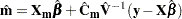
where $\text{[math]}$ represents a hypothetical realization of a missing data vector with associated design matrix $\text{[math]}$ . The matrix $\text{[math]}$ is the model-based covariance matrix between $\text{[math]}$ and the observed data $\text{[math]}$ , and other notation is as presented in the section Mixed Models Theory.

The estimated prediction variance is as follows:

	$\text{[math]}$	$\text{[math]}$
	$\text{[math]}$	$\text{[math]}$

where $\text{[math]}$ is the model-based variance matrix of $\text{[math]}$ . For further details, see Henderson (1984) and Harville (1990). This feature can be useful for forecasting time series or for computing spatial predictions.

By default, all variables from the input data set are included in the OUTP= data set. You can select a subset of these variables by using the ID statement.

OUTPM=SAS-data-set

OUTPREDM=SAS-data-set

specifies an output data set containing predicted means and related quantities. This option replaces the PM option from SAS 6.

The output data set is of the same form as that resulting from the OUTP= option, except that the predicted values do not incorporate the EBLUP values $\text{[math]}$ . They also do not use the EBLUPs for specifications that have a REPEATED statement with the SUBJECT= option and missing dependent variables. The predicted values are formed as $\text{[math]}$ in the OUTPM= data set, and standard errors are quadratic forms in the approximate variance-covariance matrix of $\text{[math]}$ as displayed by the COVB option.

By default, all variables from the input data set are included in the OUTPM= data set. You can select a subset of these variables by using the ID statement.

RESIDUAL

requests that Pearson-type and (internally) studentized residuals be added to the OUTP= and OUTPM= data sets. Studentized residuals are raw residuals standardized by their estimated standard error. When residuals are internally studentized, the data point in question has contributed to the estimation of the covariance parameter estimates on which the standard error of the residual is based. Externally studentized marginal residuals can be computed with the INFLUENCE option. Pearson-type residuals scale the residual by the standard deviation of the response.

The option has no effect unless the OUTP= or OUTPM= option is specified or unless ODS Graphics is enabled. For general information about ODS Graphics, see Chapter 21, Statistical Graphics Using ODS. For specific information about the graphics available in the MIXED procedure, see the section ODS Graphics. For computational details about studentized and Pearson residuals in MIXED, see the section Residual Diagnostics.

SINGCHOL=number

tunes the sensitivity in computing Cholesky roots. If a diagonal pivot element is less than $\text{[math]}$ *number as PROC MIXED performs the Cholesky decomposition on a matrix, the associated column is declared to be linearly dependent upon previous columns and is set to $\text{[math]}$ . The value $\text{[math]}$ is the original diagonal element of the matrix. The default for number is 1E4 times the machine epsilon; this product is approximately 1E $\text{[math]}$ 12 on most computers.

SINGRES=number

sets the tolerance for which the residual variance is considered to be zero. The default is 1E4 times the machine epsilon; this product is approximately 1E $\text{[math]}$ 12 on most computers.

SINGULAR=number

tunes the sensitivity in sweeping. If a diagonal pivot element is less than $\text{[math]}$ *number as PROC MIXED sweeps a matrix, the associated column is declared to be linearly dependent upon previous columns, and the associated parameter is set to 0. The value $\text{[math]}$ is the original diagonal element of the matrix. The default is 1E4 times the machine epsilon; this product is approximately 1E $\text{[math]}$ 12 on most computers.

SOLUTION

S

requests that a solution for the fixed-effects parameters be produced. Using notation from the section Mixed Models Theory, the fixed-effects parameter estimates are $\text{[math]}$ and their approximate standard errors are the square roots of the diagonal elements of $\text{[math]}$ . You can output this approximate variance matrix with the COVB option or modify it with the EMPIRICAL option in the PROC MIXED statement or the DDFM=KENWARDROGER option in the MODEL statement.

Along with the estimates and their approximate standard errors, a t statistic is computed as the estimate divided by its standard error. The degrees of freedom for this t statistic matches the one appearing in the "Tests of Fixed Effects" table under the effect containing the parameter. The "Pr > |t|" column contains the two-tailed $\text{[math]}$ -value corresponding to the t statistic and associated degrees of freedom. You can use the CL option to request confidence intervals for all of the parameters; they are constructed around the estimate by using a radius of the standard error times a percentage point from the t distribution.

VCIRY

requests that responses and marginal residuals be scaled by the inverse Cholesky root of the marginal variance-covariance matrix. The variables ScaledDep and ScaledResid are added to the OUTPM= data set. These quantities can be important in bootstrapping of data or residuals. Examination of the scaled residuals is also helpful in diagnosing departures from normality. Notice that the results of this scaling operation can depend on the order in which the MIXED procedure processes the data.

The VCIRY option has no effect unless you also use the OUTPM= option or unless ODS Graphics is enabled. For general information about ODS Graphics, see Chapter 21, Statistical Graphics Using ODS. For specific information about the graphics available in the MIXED procedure, see the section ODS Graphics.

XPVIX

is an alias for the COVBI option.

XPVIXI

is an alias for the COVB option.

ZETA=number

tunes the sensitivity in forming Type 3 functions. Any element in the estimable function basis with an absolute value less than number is set to 0. The default is 1E $\text{[math]}$ 8.