The MIXED Procedure

Marginal and Conditional Residuals

The marginal and conditional means in the linear mixed model are and , respectively. Accordingly, the vector of marginal residuals is defined as

and the vector of conditional residuals is

Following Gregoire, Schabenberger, and Barrett (1995), let and . Then

For an individual observation the raw, studentized, and Pearson-type residuals computed by the MIXED procedure are given in Table 58.21.

When the OUTPM= option is specified in addition to the RESIDUAL option in the MODEL statement, and are added to the data set as variables Resid, StudentResid, and PearsonResid, respectively. When the OUTP= option is specified, and are added to the data set. Raw residuals are part of the OUTPM= and OUTP= data sets without the RESIDUAL option.

Scaled Residuals

For correlated data, a set of scaled quantities can be defined through the Cholesky decomposition of the variance-covariance matrix. Since fitted residuals in linear models are rank-deficient, it is customary to draw on the variance-covariance matrix of the data. If and , then has uniform dispersion and its elements are uncorrelated.

Scaled residuals in a mixed model are meaningful for quantities based on the marginal distribution of the data. Let denote the Cholesky root of , so that , and define

By analogy with other scalings, the inverse Cholesky decomposition can also be applied to the residual vector, , although is not the variance-covariance matrix of .

To diagnose whether the covariance structure of the model has been specified correctly can be difficult based on , since the inverse Cholesky transformation affects the expected value of . You can draw on as a vector of (approximately) uncorrelated data with constant mean.

When the OUTPM= option in the MODEL statement is specified in addition to the VCIRY option, is added as variable ScaledDep and is added as ScaledResid to the data set.

Basic Idea and Statistics

The general idea of quantifying the influence of one or more observations relies on computing parameter estimates based on all data points, removing the cases in question from the data, refitting the model, and computing statistics based on the change between full-data and reduced-data estimation. Influence statistics can be coarsely grouped by the aspect of estimation that is their primary target:

• overall measures compare changes in objective functions: (restricted) likelihood distance (Cook and Weisberg 1982, Ch. 5.2)

• influence on parameter estimates: Cook’s (Cook 1977, 1979), MDFFITS (Belsley, Kuh, and Welsch 1980, p. 32)

• influence on precision of estimates: CovRatio and CovTrace

• influence on fitted and predicted values: PRESS residual, PRESS statistic (Allen 1974), DFFITS (Belsley, Kuh, and Welsch 1980, p. 15)

• outlier properties: internally and externally studentized residuals, leverage

For linear models for uncorrelated data, it is not necessary to refit the model after removing a data point in order to measure the impact of an observation on the model. The change in fixed effect estimates, residuals, residual sums of squares, and the variance-covariance matrix of the fixed effects can be computed based on the fit to the full data alone. By contrast, in mixed models several important complications arise. Data points can affect not only the fixed effects but also the covariance parameter estimates on which the fixed-effects estimates depend. Furthermore, closed-form expressions for computing the change in important model quantities might not be available.

This section provides background material for the various influence diagnostics available with the MIXED procedure. See the section Mixed Models Theory for relevant expressions and definitions. The parameter vector denotes all unknown parameters in the and matrix.

The observations whose influence is being ascertained are represented by the set and referred to simply as "the observations in ." The estimate of a parameter vector, such as , obtained from all observations except those in the set is denoted . In case of a matrix , the notation represents the matrix with the rows in removed; these rows are collected in . If is symmetric, then notation implies removal of rows and columns. The vector comprises the responses of the data points being removed, and is the variance-covariance matrix of the remaining observations. When , lowercase notation emphasizes that single points are removed, such as .

Managing the Covariance Parameters

An important component of influence diagnostics in the mixed model is the estimated variance-covariance matrix . To make the dependence on the vector of covariance parameters explicit, write it as . If one parameter, , is profiled or factored out of , the remaining parameters are denoted as . Notice that in a model where is diagonal and , the parameter vector contains the ratios of each variance component and (see Wolfinger, Tobias, and Sall 1994). When ITER=0, two scenarios are distinguished:

1. If the residual variance is not profiled, either because the model does not contain a residual variance or because it is part of the Newton-Raphson iterations, then .

2. If the residual variance is profiled, then and . Influence statistics such as Cook’s and internally studentized residuals are based on , whereas externally studentized residuals and the DFFITS statistic are based on . In a random components model with uncorrelated errors, for example, the computation of involves scaling of and by the full-data estimate and multiplying the result with the reduced-data estimate .

Certain statistics, such as MDFFITS, CovRatio, and CovTrace, require an estimate of the variance of the fixed effects that is based on the reduced number of observations. For example, is evaluated at the reduced-data parameter estimates but computed for the entire data set. The matrix , on the other hand, has rows and columns corresponding to the points in removed. The resulting matrix is evaluated at the delete-case estimates.

When influence analysis is iterative, the entire vector is updated, whether the residual variance is profiled or not. The matrices to be distinguished here are , , and , with unambiguous notation.

Predicted Values, PRESS Residual, and PRESS Statistic

An unconditional predicted value is , where the vector is the th row of . The (raw) residual is given as , and the PRESS residual is

The PRESS statistic is the sum of the squared PRESS residuals,

where the sum is over the observations in .

If EFFECT=, SIZE=, or KEEP= is not specified, PROC MIXED computes the PRESS residual for each observation selected through SELECT= (or all observations if SELECT= is not given). If EFFECT=, SIZE=, or KEEP= is specified, the procedure computes .

Leverage

For the general mixed model, leverage can be defined through the projection matrix that results from a transformation of the model with the inverse of the Cholesky decomposition of , or through an oblique projector. The MIXED procedure follows the latter path in the computation of influence diagnostics. The leverage value reported for the th observation is the th diagonal entry of the matrix

which is the weight of the observation in contributing to its own predicted value, .

While is idempotent, it is generally not symmetric and thus not a projection matrix in the narrow sense.

The properties of these leverages are generalizations of the properties in models with diagonal variance-covariance matrices. For example, , and in a model with intercept and , the leverage values

are and 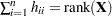. The lower bound for is achieved in an intercept-only model, and the upper bound is achieved in a saturated model. The trace of equals the rank of .

If denotes the element in row , column of , then for a model containing only an intercept the diagonal elements of are

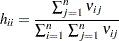Because is a sum of elements in the th row of the inverse variance-covariance matrix, can be negative, even if the correlations among data points are nonnegative. In case of a saturated model with , .

Internally and Externally Studentized Residuals

See the section Residual Diagnostics for the distinction between standardization, studentization, and scaling of residuals. Internally studentized marginal and conditional residuals are computed with the RESIDUAL option of the MODEL statement. The INFLUENCE option computes internally and externally studentized marginal residuals.

The computation of internally studentized residuals relies on the diagonal entries of , where . Externally studentized residuals require iterative influence analysis or a profiled residual variance. In the former case the studentization is based on ; in the latter case it is based on .

Cook’s

Cook’s statistic is an invariant norm that measures the influence of observations in on a vector of parameter estimates (Cook 1977). In case of the fixed-effects coefficients, let

Then the MIXED procedure computes

where is the matrix that results from sweeping .

If is known, Cook’s can be calibrated according to a chi-square distribution with degrees of freedom equal to the rank of (Christensen, Pearson, and Johnson 1992). For estimated the calibration can be carried out according to an distribution. To interpret on a familiar scale, Cook (1979) and Cook and Weisberg (1982, p. 116) refer to the 50th percentile of the reference distribution. If is equal to that percentile, then removing the points in moves the fixed-effects coefficient vector from the center of the confidence region to the 50% confidence ellipsoid (Myers 1990, p. 262).

In the case of iterative influence analysis, the MIXED procedure also computes a -type statistic for the covariance parameters. If is the asymptotic variance-covariance matrix of , then MIXED computes

DFFITS and MDFFITS

A DFFIT measures the change in predicted values due to removal of data points. If this change is standardized by the externally estimated standard error of the predicted value in the full data, the DFFITS statistic of Belsley, Kuh, and Welsch (1980, p. 15) results:

The MIXED procedure computes DFFITS when the EFFECT= or SIZE= modifier of the INFLUENCE option is not in effect. In general, an external estimate of the estimated standard error is used. When ITER > 0, the estimate is

When ITER=0 and is profiled, then

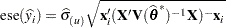When the EFFECT=, SIZE=, or KEEP= modifier is specified, the MIXED procedure computes a multivariate version suitable for the deletion of multiple data points. The statistic, termed MDFFITS after the MDFFIT statistic of Belsley, Kuh, and Welsch (1980, p. 32), is closely related to Cook’s . Consider the case so that

and let be an estimate of that does not use the observations in . The MDFFITS statistic is then computed as

If ITER=0 and is profiled, then is obtained by sweeping

The underlying idea is that if were known, then

would be in a generalized least squares regression with all but the data in .

In the case of iterative influence analysis, is evaluated at . Furthermore, a MDFFITS-type statistic is then computed for the covariance parameters:

Covariance Ratio and Trace

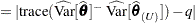
These statistics depend on the availability of an external estimate of , or at least of . Whereas Cook’s and MDFFITS measure the impact of data points on a vector of parameter estimates, the covariance-based statistics measure impact on their precision. Following Christensen, Pearson, and Johnson (1992), the MIXED procedure computes

where denotes the determinant of the nonsingular part of matrix .

In the case of iterative influence analysis these statistics are also computed for the covariance parameter estimates. If denotes the rank of , then

Likelihood Distances

The log-likelihood function and restricted log-likelihood function of the linear mixed model are given in the section Estimating Covariance Parameters in the Mixed Model. Denote as the collection of all parameters, i.e., the fixed effects and the covariance parameters . Twice the difference between the (restricted) log-likelihood evaluated at the full-data estimates and at the reduced-data estimates is known as the (restricted) likelihood distance:

Cook and Weisberg (1982, Ch. 5.2) refer to these differences as likelihood distances, Beckman, Nachtsheim, and Cook (1987) call the measures likelihood displacements. If the number of elements in that are subject to updating following point removal is , then likelihood displacements can be compared against cutoffs from a chi-square distribution with degrees of freedom. Notice that this reference distribution does not depend on the number of observations removed from the analysis, but rather on the number of model parameters that are updated. The likelihood displacement gives twice the amount by which the log likelihood of the full data changes if one were to use an estimate based on fewer data points. It is thus a global, summary measure of the influence of the observations in jointly on all parameters.

Unless METHOD=ML, the MIXED procedure computes the likelihood displacement based on the residual (=restricted) log likelihood, even if METHOD=MIVQUE0 or METHOD=TYPE1, TYPE2, or TYPE3.

Noniterative Update Formulas

Update formulas that do not require refitting of the model are available for the cases where , is known, or is known. When ITER=0 and these update formulas can be invoked, the MIXED procedure uses the computational devices that are outlined in the following paragraphs. It is then assumed that the variance-covariance matrix of the fixed effects has the form . When DDFM=KENWARDROGER, this is not the case; the estimated variance-covariance matrix is then inflated to better represent the uncertainty in the estimated covariance parameters. Influence statistics when DDFM=KENWARDROGER should iteratively update the covariance parameters (ITER > 0). The dependence of on is suppressed in the sequel for brevity.

Updating the Fixed Effects

Denote by the matrix that is assembled from columns of the identity matrix. Each column of corresponds to the removal of one data point. The point being targeted by the th column of corresponds to the row in which a appears. Furthermore, define

The change in the fixed-effects estimates following removal of the observations in is

Using results in Cook and Weisberg (1982, A2) you can further compute

If is of rank , then is deficient in rank and the MIXED procedure computes needed quantities in by sweeping (Goodnight 1979). If the rank of the matrix is less than , the removal of the observations introduces a new singularity, whether is of full rank or not. The solution vectors and then do not have the same expected values and should not be compared. When the MIXED procedure encounters this situation, influence diagnostics that depend on the choice of generalized inverse are not computed. The procedure also monitors the singularity criteria when sweeping the rows of and of . If a new singularity is encountered or a former singularity disappears, no influence statistics are computed.

Residual Variance

When is profiled out of the marginal variance-covariance matrix, a closed-form estimate of that is based on only the remaining observations can be computed provided is known. Hurtado (1993, Thm. 5.2) shows that

and . In the case of maximum likelihood estimation and for REML estimation . The constant equals the rank of for REML estimation and the number of effective observations that are removed if METHOD=ML.

Likelihood Distances

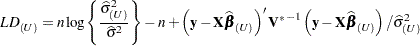
For noniterative methods the following computational devices are used to compute (restricted) likelihood distances provided that the residual variance is profiled.

The log likelihood function evaluated at the full-data and reduced-data estimates can be written as

Notice that evaluates the log likelihood for data points at the reduced-data estimates. It is not the log likelihood obtained by fitting the model to the reduced data. The likelihood distance is then

Expressions for in noniterative influence analysis are derived along the same lines.