The MIXED Procedure

Matrix Notation

Suppose that you observe data points and that you want to explain them by using values for each of explanatory variables , , . The values can be either regression-type continuous variables or dummy variables indicating class membership. The standard linear model for this setup is

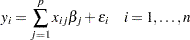where are unknown fixed-effects parameters to be estimated and are unknown independent and identically distributed normal (Gaussian) random variables with mean 0 and variance .

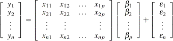
The preceding equations can be written simultaneously by using vectors and a matrix, as follows:

For convenience, simplicity, and extendability, this entire system is written as

where denotes the vector of observed ’s, is the known matrix of ’s, is the unknown fixed-effects parameter vector, and is the unobserved vector of independent and identically distributed Gaussian random errors.

In addition to denoting data, random variables, and explanatory variables in the preceding fashion, the subsequent development makes use of basic matrix operators such as transpose (), inverse (), generalized inverse (), determinant (), and matrix multiplication. See Searle (1982) for details about these and other matrix techniques.

Formulation of the Mixed Model

The previous general linear model is certainly a useful one (Searle 1971), and it is the one fitted by the GLM procedure. However, many times the distributional assumption about is too restrictive. The mixed model extends the general linear model by allowing a more flexible specification of the covariance matrix of . In other words, it allows for both correlation and heterogeneous variances, although you still assume normality.

The mixed model is written as

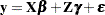where everything is the same as in the general linear model except for the addition of the known design matrix, , and the vector of unknown random-effects parameters, . The matrix can contain either continuous or dummy variables, just like . The name mixed model comes from the fact that the model contains both fixed-effects parameters, , and random-effects parameters, . See Henderson (1990) and Searle, Casella, and McCulloch (1992) for historical developments of the mixed model.

A key assumption in the foregoing analysis is that and are normally distributed with

The variance of is, therefore, . You can model by setting up the random-effects design matrix and by specifying covariance structures for and .

Note that this is a general specification of the mixed model, in contrast to many texts and articles that discuss only simple random effects. Simple random effects are a special case of the general specification with containing dummy variables, containing variance components in a diagonal structure, and , where denotes the identity matrix. The general linear model is a further special case with and .

The following two examples illustrate the most common formulations of the general linear mixed model.

Example: Growth Curve with Compound Symmetry

Suppose that you have three growth curve measurements for individuals and that you want to fit an overall linear trend in time. Your matrix is as follows:

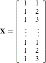The first column (coded entirely with s) fits an intercept, and the second column (coded with times of ) fits a slope. Here, and .

Suppose further that you want to introduce a common correlation among the observations from a single individual, with correlation being the same for all individuals. One way of setting this up in the general mixed model is to eliminate the and matrices and let the matrix be block diagonal with blocks corresponding to the individuals and with each block having the compound-symmetry structure. This structure has two unknown parameters, one modeling a common covariance and the other modeling a residual variance. The form for would then be as follows:

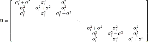where blanks denote zeros. There are rows and columns altogether, and the common correlation is .

The PROC MIXED statements to fit this model are as follows:

proc mixed;
   class indiv;
   model y = time;
   repeated / type=cs subject=indiv;
run;

Here, indiv is a classification variable indexing individuals. The MODEL statement fits a straight line for time ; the intercept is fit by default just as in PROC GLM. The REPEATED statement models the matrix: TYPE=CS specifies the compound symmetry structure, and SUBJECT=INDIV specifies the blocks of .

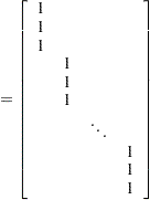
An alternative way of specifying the common intra-individual correlation is to let

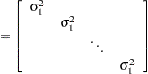and . The matrix has rows and columns, and is .

You can set up this model in PROC MIXED in two different but equivalent ways:

proc mixed;
   class indiv;
   model y = time;
   random indiv;
run;

proc mixed;
   class indiv;
   model y = time;
   random intercept / subject=indiv;
run;

Both of these specifications fit the same model as the previous one that used the REPEATED statement; however, the RANDOM specifications constrain the correlation to be positive, whereas the REPEATED specification leaves the correlation unconstrained.

Example: Split-Plot Design

The split-plot design involves two experimental treatment factors, A and B, and two different sizes of experimental units to which they are applied (see Winer 1971, Snedecor and Cochran 1980, Milliken and Johnson 1992, and Steel, Torrie, and Dickey 1997). The levels of A are randomly assigned to the larger-sized experimental unit, called whole plots, whereas the levels of B are assigned to the smaller-sized experimental unit, the subplots. The subplots are assumed to be nested within the whole plots, so that a whole plot consists of a cluster of subplots and a level of A is applied to the entire cluster.

Such an arrangement is often necessary by nature of the experiment, the classical example being the application of fertilizer to large plots of land and different crop varieties planted in subdivisions of the large plots. For this example, fertilizer is the whole-plot factor A and variety is the subplot factor B.

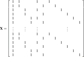
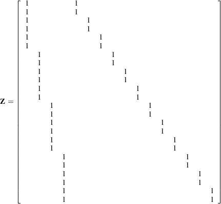
The first example is a split-plot design for which the whole plots are arranged in a randomized block design. The appropriate PROC MIXED statements are as follows:

proc mixed;
   class a b block;
   model y = a|b;
   random block a*block;
run;

Here

and , , and have the following form:

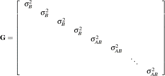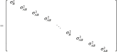
where is the variance component for Block and is the variance component for A*Block. Changing the RANDOM statement as follows fits the same model, but with and sorted differently:

random int a / subject=block;

Estimating Covariance Parameters in the Mixed Model

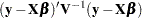
Estimation is more difficult in the mixed model than in the general linear model. Not only do you have as in the general linear model, but you have unknown parameters in , , and as well. Least squares is no longer the best method. Generalized least squares (GLS) is more appropriate, minimizing

However, it requires knowledge of and, therefore, knowledge of and . Lacking such information, one approach is to use estimated GLS, in which you insert some reasonable estimate for into the minimization problem. The goal thus becomes finding a reasonable estimate of and .

In many situations, the best approach is to use likelihood-based methods, exploiting the assumption that and are normally distributed (Hartley and Rao 1967; Patterson and Thompson 1971; Harville 1977; Laird and Ware 1982; Jennrich and Schluchter 1986). PROC MIXED implements two likelihood-based methods: maximum likelihood (ML) and restricted/residual maximum likelihood (REML). A favorable theoretical property of ML and REML is that they accommodate data that are missing at random (Rubin 1976; Little 1995).

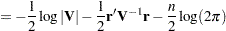
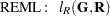
PROC MIXED constructs an objective function associated with ML or REML and maximizes it over all unknown parameters. Using calculus, it is possible to reduce this maximization problem to one over only the parameters in and . The corresponding log-likelihood functions are as follows:

where and is the rank of . PROC MIXED actually minimizes times these functions by using a ridge-stabilized Newton-Raphson algorithm. Lindstrom and Bates (1988) provide reasons for preferring Newton-Raphson to the Expectation-Maximum (EM) algorithm described in Dempster, Laird, and Rubin (1977) and Laird, Lange, and Stram (1987), as well as analytical details for implementing a QR-decomposition approach to the problem. Wolfinger, Tobias, and Sall (1994) present the sweep-based algorithms that are implemented in PROC MIXED.

One advantage of using the Newton-Raphson algorithm is that the second derivative matrix of the objective function evaluated at the optima is available upon completion. Denoting this matrix , the asymptotic theory of maximum likelihood (see Serfling 1980) shows that is an asymptotic variance-covariance matrix of the estimated parameters of and . Thus, tests and confidence intervals based on asymptotic normality can be obtained. However, these can be unreliable in small samples, especially for parameters such as variance components that have sampling distributions that tend to be skewed to the right.

If a residual variance is a part of your mixed model, it can usually be profiled out of the likelihood. This means solving analytically for the optimal and plugging this expression back into the likelihood formula (see Wolfinger, Tobias, and Sall 1994). This reduces the number of optimization parameters by one and can improve convergence properties. PROC MIXED profiles the residual variance out of the log likelihood whenever it appears reasonable to do so. This includes the case when equals and when it has blocks with a compound symmetry, time series, or spatial structure. PROC MIXED does not profile the log likelihood when has unstructured blocks, when you use the HOLD= or NOITER option in the PARMS statement, or when you use the NOPROFILE option in the PROC MIXED statement.

Instead of ML or REML, you can use the noniterative MIVQUE0 method to estimate and (Rao 1972; LaMotte 1973; Wolfinger, Tobias, and Sall 1994). In fact, by default PROC MIXED uses MIVQUE0 estimates as starting values for the ML and REML procedures. For variance component models, another estimation method involves equating Type 1, 2, or 3 expected mean squares to their observed values and solving the resulting system. However, Swallow and Monahan (1984) present simulation evidence favoring REML and ML over MIVQUE0 and other method-of-moment estimators.

Estimating Fixed and Random Effects in the Mixed Model

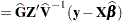
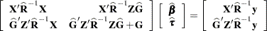
ML, REML, MIVQUE0, or Type1–Type3 provide estimates of and , which are denoted and , respectively. To obtain estimates of and , the standard method is to solve the mixed model equations (Henderson 1984):

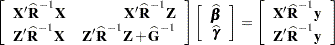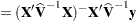
The solutions can also be written as

and have connections with empirical Bayes estimators (Laird and Ware 1982, Carlin and Louis 1996).

Note that the mixed model equations are extended normal equations and that the preceding expression assumes that is nonsingular. For the extreme case where the eigenvalues of are very large, contributes very little to the equations and is close to what it would be if actually contained fixed-effects parameters. On the other hand, when the eigenvalues of are very small, dominates the equations and is close to . For intermediate cases, can be viewed as shrinking the fixed-effects estimates of toward (Robinson 1991).

If is singular, then the mixed model equations are modified (Henderson 1984) as follows:

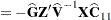
Denote the generalized inverses of the nonsingular and singular forms of the mixed model equations by and , respectively. In the nonsingular case, the solution estimates the random effects directly, but in the singular case the estimates of random effects are achieved through a back-transformation where is the solution to the modified mixed model equations. Similarly, while in the nonsingular case itself is the estimated covariance matrix for , in the singular case the covariance estimate for is given by where

An example of when the singular form of the equations is necessary is when a variance component estimate falls on the boundary constraint of .

Model Selection

The previous section on estimation assumes the specification of a mixed model in terms of , , , and . Even though and have known elements, their specific form and construction are flexible, and several possibilities can present themselves for a particular data set. Likewise, several different covariance structures for and might be reasonable.

Space does not permit a thorough discussion of model selection, but a few brief comments and references are in order. First, subject matter considerations and objectives are of great importance when selecting a model; see Diggle (1988) and Lindsey (1993).

Second, when the data themselves are looked to for guidance, many of the graphical methods and diagnostics appropriate for the general linear model extend to the mixed model setting as well (Christensen, Pearson, and Johnson 1992).

Finally, a likelihood-based approach to the mixed model provides several statistical measures for model adequacy as well. The most common of these are the likelihood ratio test and Akaike’s and Schwarz’s criteria (Bozdogan 1987; Wolfinger 1993; Keselman et al. 1998, 1999).

Statistical Properties

If and are known, is the best linear unbiased estimator (BLUE) of , and is the best linear unbiased predictor (BLUP) of (Searle 1971; Harville 1988, 1990; Robinson 1991; McLean, Sanders, and Stroup 1991). Here, "best" means minimum mean squared error. The covariance matrix of is

where denotes a generalized inverse (see Searle 1971).

However, and are usually unknown and are estimated by using one of the aforementioned methods. These estimates, and , are therefore simply substituted into the preceding expression to obtain

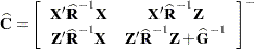as the approximate variance-covariance matrix of ). In this case, the BLUE and BLUP acronyms no longer apply, but the word empirical is often added to indicate such an approximation. The appropriate acronyms thus become EBLUE and EBLUP.

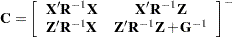
McLean and Sanders (1988) show that can also be written as

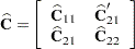where

Note that is the familiar estimated generalized least squares formula for the variance-covariance matrix of .

As a cautionary note, tends to underestimate the true sampling variability of
() because no account is made for the uncertainty in estimating and . Although inflation factors have been proposed (Kackar and Harville 1984; Kass and Steffey 1989; Prasad and Rao 1990), they tend to be small for data sets that are fairly well balanced. PROC MIXED does not compute any inflation factors by default, but rather accounts for the downward bias by using the approximate and statistics described subsequently. The DDFM=KENWARDROGER option in the MODEL statement prompts PROC MIXED to compute a specific inflation factor along with Satterthwaite-based degrees of freedom.

Inference and Test Statistics

For inferences concerning the covariance parameters in your model, you can use likelihood-based statistics. One common likelihood-based statistic is the Wald , which is computed as the parameter estimate divided by its asymptotic standard error. The asymptotic standard errors are computed from the inverse of the second derivative matrix of the likelihood with respect to each of the covariance parameters. The Wald is valid for large samples, but it can be unreliable for small data sets and for parameters such as variance components, which are known to have a skewed or bounded sampling distribution.

A better alternative is the likelihood ratio statistic. This statistic compares two covariance models, one a special case of the other. To compute it, you must run PROC MIXED twice, once for each of the two models, and then subtract the corresponding values of times the log likelihoods. You can use either ML or REML to construct this statistic, which tests whether the full model is necessary beyond the reduced model.

As long as the reduced model does not occur on the boundary of the covariance parameter space, the statistic computed in this fashion has a large-sample distribution that is with degrees of freedom equal to the difference in the number of covariance parameters between the two models. If the reduced model does occur on the boundary of the covariance parameter space, the asymptotic distribution becomes a mixture of distributions (Self and Liang 1987). A common example of this is when you are testing that a variance component equals its lower boundary constraint of 0.

A final possibility for obtaining inferences concerning the covariance parameters is to simulate or resample data from your model and construct empirical sampling distributions of the parameters. The SAS macro language and the ODS system are useful tools in this regard.

F and t Tests for Fixed- and Random-Effects Parameters

For inferences concerning the fixed- and random-effects parameters in the mixed model, consider estimable linear combinations of the following form:

The estimability requirement (Searle 1971) applies only to the portion of , because any linear combination of is estimable. Such a formulation in terms of a general matrix encompasses a wide variety of common inferential procedures such as those employed with Type 1–Type 3 tests and LS-means. The CONTRAST and ESTIMATE statements in PROC MIXED enable you to specify your own matrices. Typically, inference on fixed effects is the focus, and, in this case, the portion of is assumed to contain all 0s.

Statistical inferences are obtained by testing the hypothesis

or by constructing point and interval estimates.

When consists of a single row, a general t statistic can be constructed as follows (see McLean and Sanders 1988, Stroup 1989a):

Under the assumed normality of and , t has an exact t distribution only for data exhibiting certain types of balance and for some special unbalanced cases. In general, t is only approximately t-distributed, and its degrees of freedom must be estimated. See the DDFM= option for a description of the various degrees-of-freedom methods available in PROC MIXED.

With being the approximate degrees of freedom, the associated confidence interval is

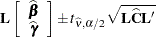where is the th percentile of the distribution.

When the rank of is greater than 1, PROC MIXED constructs the following general F statistic:

where . Analogous to t, F in general has an approximate F distribution with numerator degrees of freedom and denominator degrees of freedom.

The t and F statistics enable you to make inferences about your fixed effects, which account for the variance-covariance model you select. An alternative is the statistic associated with the likelihood ratio test. This statistic compares two fixed-effects models, one a special case of the other. It is computed just as when comparing different covariance models, although you should use ML and not REML here because the penalty term associated with restricted likelihoods depends upon the fixed-effects specification.

F Tests With the ANOVAF Option

The ANOVAF option computes F tests by the following method in models with REPEATED statement and without RANDOM statement. Let denote the matrix of estimable functions for the hypothesis , where are the fixed-effects parameters. Let , and suppose that denotes the estimated variance-covariance matrix of (see the section Statistical Properties for the construction of ).

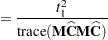
The ANOVAF F statistics are computed as

Notice that this is a modification of the usual F statistic where is replaced with and is replaced with ; see, for example, Brunner, Domhof, and Langer (2002, Sec. 5.4). The p-values for this statistic are computed from either an or an distribution. The respective degrees of freedom are determined by the MIXED procedure as follows:

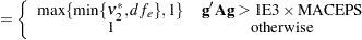The term in the term for the denominator degrees of freedom is based on approximating based on a first-order Taylor series about the true covariance parameters. This generalizes results in the appendix of Brunner, Dette, and Munk (1997) to a broader class of models. The vector contains the partial derivatives

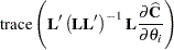and is the asymptotic variance-covariance matrix of the covariance parameter estimates (ASYCOV option).

PROC MIXED reports and as "NumDF" and "DenDF" under the "ANOVA F" heading in the output. The corresponding p-values are denoted as "Pr > F(DDF)" for and "Pr > F(infty)" for , respectively.

P-values computed with the ANOVAF option can be identical to the nonparametric tests in Akritas, Arnold, and Brunner (1997) and in Brunner, Domhof, and Langer (2002), provided that the response data consist of properly created (and sorted) ranks and that the covariance parameters are estimated by MIVQUE0 in models with REPEATED statement and properly chosen SUBJECT= and/or GROUP= effects.

If you model an unstructured covariance matrix in a longitudinal model with one or more repeated factors, the ANOVAF results are identical to a multivariate MANOVA where degrees of freedom are corrected with the Greenhouse-Geiser adjustment (Greenhouse and Geiser 1959). For example, suppose that factor A has 2 levels and factor B has 4 levels. The following two sets of statements produce the same p-values:

proc mixed data=Mydata anovaf method=mivque0;
   class id A B;
   model score = A | B / chisq;
   repeated / type=un subject=id;
   ods select Tests3;
run;

proc transpose data=MyData out=tdata;
   by id;
   var score;
proc glm data=tdata;
   model col: = / nouni;
   repeated A 2, B 4;
   ods output ModelANOVA=maov epsilons=eps;
run;
proc transpose data=eps(where=(substr(statistic,1,3)='Gre')) out=teps;
  var cvalue1;
run;

data aov; set maov;
  if (_n_ = 1) then merge teps;
  if (Source='A') then do;
      pFddf = ProbF;
      pFinf = 1 - probchi(df*Fvalue,df);
      output;
  end; else if (Source='B') then do;
      pFddf = ProbFGG;
      pFinf = 1 - probchi(df*col1*Fvalue,df*col1);
      output;
  end; else if (Source='A*B') then do;
      pfddF = ProbFGG;
      pFinf = 1 - probchi(df*col2*Fvalue,df*col2);
      output;
  end;
proc print data=aov label noobs;
  label Source = 'Effect'
        df     = 'NumDF'
        Fvalue = 'Value'
        pFddf  = 'Pr > F(DDF)'
        pFinf  = 'Pr > F(infty)';
  var Source df Fvalue pFddf pFinf;
  format pF: pvalue6.;
run;

The PROC GLM code produces p-values that correspond to the ANOVAF p-values shown as Pr > F(DDF) in the MIXED output. The subsequent DATA step computes the p-values that correspond to Pr > F(infty) in the PROC MIXED output.