The MIXED Procedure

| PROC MIXED Statement |
The PROC MIXED statement invokes the procedure. Table 58.2 summarizes important options in the PROC MIXED statement by function. These and other options in the PROC MIXED statement are then described fully in alphabetical order.
Option |
Description |
|---|---|
Basic Options |
|
Specifies input data set |
|
Specifies the estimation method |
|
Includes scale parameter in optimization |
|
Determines the sort order of CLASS variables |
|
Displayed Output |
|
Displays asymptotic correlation matrix of covariance parameter estimates |
|
Displays asymptotic covariance matrix of covariance parameter estimates |
|
Requests confidence limits for covariance parameter estimates |
|
Displays asymptotic standard errors and Wald tests for covariance parameters |
|
Displays a table of information criteria |
|
Displays estimates and gradients added to "Iteration History" |
|
Writes periodic status notes to the log |
|
Displays mixed model equations |
|
Displays the solution to the mixed model equations |
|
Suppresses "Class Level Information" completely or in parts |
|
Suppresses "Iteration History" table |
|
Produces ODS statistical graphics |
|
Produces ratio of covariance parameter estimates with residual variance |
|
Optimization Options |
|
Specifies the maximum number of likelihood evaluations |
|
Specifies the maximum number of iterations |
|
Computational Options |
|
Requests and tunes the relative function convergence criterion |
|
Requests and tunes the relative gradient convergence criterion |
|
Requests and tunes the relative Hessian convergence criterion |
|
Selects between-within degree of freedom method |
|
Computes empirical ("sandwich") estimators |
|
Unbounds covariance parameter estimates |
|
Specifies starting value for minimum ridge value |
|
Applies Fisher scoring where applicable |
|
You can specify the following options.
- ABSOLUTE
makes the convergence criterion absolute. By default, it is relative (divided by the current objective function value). See the CONVF, CONVG, and CONVH options in this section for a description of various convergence criteria.
- ALPHA=number
requests that confidence limits be constructed for the covariance parameter estimates with confidence level
 . The value of number must be between 0 and 1; the default is 0.05.
 - ANOVAF
The ANOVAF option computes F tests in models with REPEATED statement and without RANDOM statement by a method similar to that of Brunner, Domhof, and Langer (2002). The method consists of computing special F statistics and adjusting their degrees of freedom. The technique is a generalization of the Greenhouse-Geiser adjustment in MANOVA models (Greenhouse and Geiser 1959). For more details, see the section F Tests With the ANOVAF Option.
- ASYCORR
produces the asymptotic correlation matrix of the covariance parameter estimates. It is computed from the corresponding asymptotic covariance matrix (see the description of the ASYCOV option, which follows). For ODS purposes, the name of the "Asymptotic Correlation" table is "AsyCorr."
- ASYCOV
requests that the asymptotic covariance matrix of the covariance parameters be displayed. By default, this matrix is the observed inverse Fisher information matrix, which equals
 , where
  is the Hessian (second derivative) matrix of the objective function. See the section Covariance Parameter Estimates for more information about this matrix. When you use the SCORING= option and PROC MIXED converges without stopping the scoring algorithm, PROC MIXED uses the expected Hessian matrix to compute the covariance matrix instead of the observed Hessian. For ODS purposes, the name of the "Asymptotic Covariance" table is "AsyCov."
 - CL<=WALD>
-
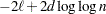
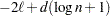
requests confidence limits for the covariance parameter estimates. A Satterthwaite approximation is used to construct limits for all parameters that have a lower boundary constraint of zero. These limits take the form
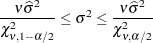
where
 ,
,  is the Wald statistic
  , and the denominators are quantiles of the
  -distribution with
  degrees of freedom. See Milliken and Johnson (1992) and Burdick and Graybill (1992) for similar techniques.
 For all other parameters, Wald
-scores and normal quantiles are used to construct the limits. Wald limits are also provided for variance components if you specify the NOBOUND option. The optional =WALD specification requests Wald limits for all parameters. The confidence limits are displayed as extra columns in the "Covariance Parameter Estimates" table. The confidence level is
 by default; this can be changed with the ALPHA= option.
 - CONVF<=number>
-
requests the relative function convergence criterion with tolerance number. The relative function convergence criterion is
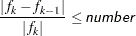
where
 is the value of the objective function at iteration k. To prevent the division by
  , use the ABSOLUTE option. The default convergence criterion is CONVH, and the default tolerance is 1E
 8.
8. - CONVG <=number>
-
requests the relative gradient convergence criterion with tolerance number. The relative gradient convergence criterion is
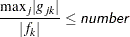
where
is the value of the objective function, and  is the
  th element of the gradient (first derivative) of the objective function, both at iteration k. To prevent division by , use the ABSOLUTE option. The default convergence criterion is CONVH, and the default tolerance is 1E8.
 - CONVH<=number>
-
requests the relative Hessian convergence criterion with tolerance number. The relative Hessian convergence criterion is

where
is the value of the objective function,  is the gradient (first derivative) of the objective function, and
  is the Hessian (second derivative) of the objective function, all at iteration
  .
. If
is singular, then PROC MIXED uses the following relative criterion: 
To prevent the division by
, use the ABSOLUTE option. The default convergence criterion is CONVH, and the default tolerance is 1E8. - COVTEST
-
produces asymptotic standard errors and Wald
-tests for the covariance parameter estimates. - DATA=SAS-data-set
names the SAS data set to be used by PROC MIXED. The default is the most recently created data set.
- DFBW
has the same effect as the DDFM=BW option in the MODEL statement.
- EMPIRICAL
-
computes the estimated variance-covariance matrix of the fixed-effects parameters by using the asymptotically consistent estimator described in Huber (1967), White (1980), Liang and Zeger (1986), and Diggle, Liang, and Zeger (1994). This estimator is commonly referred to as the "sandwich" estimator, and it is computed as follows:
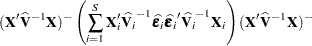
Here,
 ,
,  is the number of subjects, and matrices with an
  subscript are those for the th subject. You must include the SUBJECT= option in either a RANDOM or REPEATED statement for this option to take effect.
 When you specify the EMPIRICAL option, PROC MIXED adjusts all standard errors and test statistics involving the fixed-effects parameters. This changes output in the following tables (listed in Table 58.22): Contrast, CorrB, CovB, Diffs, Estimates, InvCovB, LSMeans, Slices, SolutionF, Tests1–Tests3. The OUTP= and OUTPM= data sets are also affected. Finally, the Satterthwaite and Kenward-Roger degrees of freedom methods are not available if you specify the EMPIRICAL option.
- IC
-
displays a table of various information criteria. The criteria are all in smaller-is-better form, and are described in Table 58.3.
Table 58.3 Information Criteria Criterion
Formula
Reference
AIC

Akaike (1974)
AICC

Hurvich and Tsai (1989)
Burnham and Anderson (1998)
HQIC
 for
for 
Hannan and Quinn (1979)
BIC
 for
for 
Schwarz (1978)
CAIC
 for
for Bozdogan (1987)
Here
 denotes the maximum value of the (possibly restricted) log likelihood,
  the dimension of the model, and
  the number of observations. In SAS 6 of SAS/STAT software, equals the number of valid observations for maximum likelihood estimation and
  for restricted maximum likelihood estimation, where
  equals the rank of
  . In later versions, equals the number of effective subjects as displayed in the "Dimensions" table, unless this value equals 1, in which case equals the number of levels of the first random effect you specify in a RANDOM statement. If the number of effective subjects equals 1 and you have no RANDOM statements, then reverts to the SAS 6 values. For AICC (a finite-sample corrected version of AIC),
  equals the SAS 6 values of , unless this number is less than
  , in which case it equals . When
  , the value of the HQIC criterion is
  . When
  , the values of the BIC and CAIC criteria are and
  , respectively.
 For restricted likelihood estimation,
equals  , the effective number of estimated covariance parameters. In SAS 6, when a parameter estimate lies on a boundary constraint, then it is still included in the calculation of , but in later versions it is not. The most common example of this behavior is when a variance component is estimated to equal zero. For maximum likelihood estimation, equals
  . The value of is displayed in the "Information Criteria" table as the value of Parms variable; see Table 58.23.
 For ODS purposes, the name of the "Information Criteria" table is "InfoCrit."
- INFO
-
is a default option. The creation of the "Model Information," "Dimensions," and "Number of Observations" tables can be suppressed by using the NOINFO option.
Note that in SAS 6 this option displays the "Model Information" and "Dimensions" tables.
- ITDETAILS
displays the parameter values at each iteration and enables the writing of notes to the SAS log pertaining to "infinite likelihood" and "singularities" during Newton-Raphson iterations.
- LOGNOTE
writes periodic notes to the log describing the current status of computations. It is designed for use with analyses requiring extensive CPU resources.
- MAXFUNC=number
specifies the maximum number of likelihood evaluations in the optimization process. The default is 150.
- MAXITER=number
specifies the maximum number of iterations. The default is 50.
-
METHOD=REML
 |ML|MIVQUE0|TYPE1|TYPE2|TYPE3
-
specifies the estimation method for the covariance parameters. The REML specification performs residual (restricted) maximum likelihood, and it is the default method. The ML specification performs maximum likelihood, and the MIVQUE0 specification performs minimum variance quadratic unbiased estimation of the covariance parameters.
The METHOD=TYPE
specifications apply only to variance component models with no SUBJECT= effects and no REPEATED statement. An analysis of variance table is included in the output, and the expected mean squares are used to estimate the variance components (see
Chapter 41,
The GLM Procedure,
for further explanation). The resulting method-of-moment variance component estimates are used in subsequent calculations, including standard errors computed from ESTIMATE and LSMEANS statements. For ODS purposes, the new table names are "Type1," "Type2," and "Type3," respectively. - MMEQ
-
requests that the coefficient matrix and the right-hand side of the mixed model equations be displayed. If
 is nonsingular, the coefficient matrix and the right-hand side have the following form:
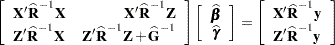
If
is singular, the coefficient matrix and right-hand side have the following modified form: 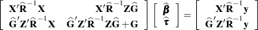
See the section Estimating Fixed and Random Effects in the Mixed Model for further information about these equations.
- MMEQSOL
-
requests that a solution to the mixed model equations be produced, in addition to the inverted coefficients matrix. If
is nonsingular, the formula is the same as the preceding description of the MMEQ option. If is singular,  and
and  are displayed in addition to the inverse of the modified coefficient matrix.
 See the section Estimating Fixed and Random Effects in the Mixed Model for further information about these equations and solution transformation.
- NAMELEN<=number>
specifies the length to which long effect names are shortened. The default and minimum value is 20.
- NOBOUND
has the same effect as the NOBOUND option in the PARMS statement.
- NOCLPRINT<=number>
suppresses the display of the "Class Level Information" table if you do not specify number. If you do specify number, only levels with totals that are less than number are listed in the table.
- NOINFO
suppresses the display of the "Model Information," "Dimensions," and "Number of Observations" tables.
- NOITPRINT
- NOPROFILE
includes the residual variance as part of the Newton-Raphson iterations. This option applies only to models that have a residual variance parameter. By default, this parameter is profiled out of the likelihood calculations, except when you have specified the HOLD= option in the PARMS statement.
- ORD
displays ordinates of the relevant distribution in addition to p-values. The ordinate can be viewed as an approximate odds ratio of hypothesis probabilities.
- ORDER=DATA | FORMATTED | FREQ | INTERNAL
-
specifies the order in which to sort the levels of the classification variables (which are specified in the CLASS statement). This option applies to the levels for all classification variables, except when you use the (default) ORDER=FORMATTED option with numeric classification variables that have no explicit format. With this option, the levels of such variables are ordered by their internal value.
The ORDER= option can take the following values:
Value of ORDER=
Levels Sorted By
DATA
Order of appearance in the input data set
FORMATTED
External formatted value, except for numeric variables with no explicit format, which are sorted by their unformatted (internal) value
FREQ
Descending frequency count; levels with the most observations come first in the order
INTERNAL
Unformatted value
By default, ORDER=FORMATTED. For ORDER=FORMATTED and ORDER=INTERNAL, the sort order is machine-dependent. For more information about sorting order, see the chapter on the SORT procedure in the Base SAS Procedures Guide and the discussion of BY-group processing in SAS Language Reference: Concepts.
- PLOTS <(global-plot-options )> <=plot-request <(options )>>
-
PLOTS <(global-plot-options )> <= (plot-request<(options)>
<...plot-request<(options)> >)> -
requests that the MIXED procedure produce statistical graphics via the Output Delivery System, provided that ODS Graphics is enabled.
ODS Graphics must be enabled before requesting plots. For example:
ods graphics on;
proc mixed data=heights plots=all;
   class Family Gender;
   model Height = Gender / residual;
   random Family Family*Gender;
run;
ods graphics off;
For more information about enabling and disabling ODS Graphics, see the section Enabling and Disabling ODS Graphics in Chapter 21, Statistical Graphics Using ODS.
For examples of the basic statistical graphics produced by the MIXED procedure and aspects of their computation and interpretation, see the section ODS Graphics.
The global-plot-options apply to all relevant plots generated by the MIXED procedure. The global-plot-options supported by the MIXED procedure follow.
Global Plot Options- OBSNO
uses the data set observation number to identify observations in tooltips, provided that the observation number can be determined. Otherwise, the number displayed in tooltips is the index of the observation as it is used in the analysis within the BY group.
- ONLY
suppresses the default plots. Only the plots specifically requested are produced.
- UNPACK
breaks a graphic that is otherwise paneled into individual component plots.
-
MAXPOINTS=NONE|number
specifies that plots with elements that require processing more than number points be suppressed. The default is MAXPOINTS=5000. No plots are suppressed if you specify MAXPOINTS=NONE.
Specific Plot OptionsThe following listing describes the specific plots and their options.
- ALL
requests that all plots appropriate for the particular analysis be produced.
- BOXPLOT <(boxplot-options)>
requests box plots for the effects in your model that consist of classification effects only. Note that these effects can involve more than one classification variable (interaction and nested effects), but they cannot contain any continuous variables. By default, the BOXPLOT request produces box plots based on (conditional) raw residuals for the qualifying effects in the MODEL, RANDOM, and REPEATED statements. See the discussion of the boxplot-options in a later section for information about how to tune your box plot request.
- DISTANCE<(USEINDEX)>
requests a plot of the likelihood or restricted likelihood distance. When influence diagnostics are requested with set selection according to an effect, the USEINDEX option enables you to replace the formatted tick values on the horizontal axis with integer indices of the effect levels in order to reduce the space taken up by the horizontal plot axis.
- INFLUENCEESTPLOT<(options)>
requests panels of the deletion estimates in an influence analysis, provided that the INFLUENCE option is specified in the MODEL statement. No plots are produced for fixed-effects parameters associated with singular columns in the
 matrix or for covariance parameters associated with singularities in the ASYCOV matrix. By default, separate panels are produced for the fixed-effects and covariance parameters delete estimates. The FIXED and RANDOM options enable you to select these specific panels. The UNPACK option produces separate plots for each of the parameter estimates. The USEINDEX option replaces formatted tick values for the horizontal axis with integer indices.
 - INFLUENCESTATPANEL<(options)>
requests panels of influence statistics. For iterative influence analysis (see the INFLUENCE option in the MODEL statement), the panel shows the Cook’s
 and CovRatio statistics for fixed-effects and covariance parameters, enabling you to gauge impact on estimates and precision for both types of estimates. In noniterative analysis, only statistics for the fixed effects are plotted. The UNPACK option produces separate plots from the elements in the panel. The USEINDEX option replaces formatted tick values for the horizontal axis with integer indices.
 - RESIDUALPANEL <(residual-plot-options)>
requests a panel of raw residuals. By default, the conditional residuals are produced. See the discussion of residual-plot-options in a later section for information about how to tune this panel.
- STUDENTPANEL <(residual-plot-options)>
requests a panel of studentized residuals. By default, the conditional residuals are produced. See the discussion of residual-plot-options in a later section for information about how to tune this panel.
- PEARSONPANEL <(residual-plot-options)>
requests a panel of Pearson residuals. By default, the conditional residuals are produced. See the discussion of residual-plot-options in a later section for information about how to tune this panel.
- PRESS<(USEINDEX)>
requests a plot of PRESS residuals or PRESS statistics. These are based on "leave-one-out" or "leave-set-out" prediction of the marginal mean. When influence diagnostics are requested with set selection according to an effect, the USEINDEX option enables you to replace the formatted tick values on the horizontal axis with integer indices of the effect levels in order to reduce the space taken up by the horizontal plot axis.
- VCIRYPANEL <(residual-plot-options)>
requests a panel of residual graphics based on the scaled residuals. See the VCIRY option in the MODEL statement for details about these scaled residuals. Only the UNPACK and BOX options of the residual-plot-options are available for this type of residual panel.
- NONE
-
suppresses all plots.
Residual Plot OptionsThe residual-plot-options determine both the composition of the panels and the type of residuals being plotted.
- BOX
- BOXPLOT
replaces the inset of summary statistics in the lower-right corner of the panel with a box plot of the residual (the "PROC GLIMMIX look").
- CONDITIONAL
- BLUP
constructs plots from conditional residuals.
- MARGINAL
- NOBLUP
constructs plots from marginal residuals.
- UNPACK
produces separate plots from the elements of the panel. The inset statistics are not part of the unpack operation.
Box Plot OptionsThe boxplot-options determine whether box plots are produced for residuals or for residuals and observed values, and for which model effects the box plots are constructed. The available boxplot-options are as follows.
- CONDITIONAL
- BLUP
constructs box plots from conditional residuals—that is, residuals using the estimated BLUPs of random effects.
- FIXED
produces box plots for all fixed effects (MODEL statement) consisting entirely of classification variables
- GROUP
produces box plots for all GROUP= effects (RANDOM and REPEATED statement) consisting entirely of classification variables
- MARGINAL
- NOBLUP
constructs box plots from marginal residuals.
- NPANEL=number
-
provides the ability to break a box plot into multiple graphics. If number is negative, no balancing of the number of boxes takes place and number is the maximum number of boxes per graphic. If number is positive, the number of boxes per graphic is balanced. For example, suppose variable A has 125 levels, and consider the following statements:
   ods graphics on;
   proc mixed plots=boxplot(npanel=20);
       class A;
       model y = A;
   run;
The box balancing results in six plots with 18 boxes each and one plot with 17 boxes. If number is zero, and this is the default, all levels of the effect are displayed in a single plot.
- OBSERVED
adds box plots of the observed data for the selected effects.
- RANDOM
produces box plots for all random effects (RANDOM statement) consisting entirely of classification variables. This does not include effects specified in the GROUP= or SUBJECT= options of the RANDOM statement.
- REPEATED
produces box plots for the repeated effects (REPEATED statement). This does not include effects specified in the GROUP= or SUBJECT= options of the REPEATED statement.
- STUDENT
constructs box plots from studentized residuals rather than from raw residuals.
- SUBJECT
produces box plots for all SUBJECT= effects (RANDOM and REPEATED statement) consisting entirely of classification variables.
- USEINDEX
uses as the horizontal axis label the index of the effect level rather than the formatted value(s). For classification variables with many levels or model effects that involve multiple classification variables, the formatted values identifying the effect levels can take up too much space as axis tick values, leading to extensive thinning. The USEINDEX option replaces tick values constructed from formatted values with the internal level number.
Multiple Plot RequestsYou can list a plot request one or more times with different options. For example, the following statements request a panel of marginal raw residuals, individual plots generated from a panel of the conditional raw residuals, and a panel of marginal studentized residuals:
ods graphics on;
proc mixed plots(only)=(
       ResidualPanel(marginal)
       ResidualPanel(unpack conditional)
       StudentPanel(marginal box));
The inset of residual statistics is replaced in this last panel by a box plot of the studentized residuals. Similarly, if you specify the INFLUENCE option in the MODEL statement, then the following statements request statistical graphics of fixed-effects deletion estimates (in a panel), covariance parameter deletion estimates (unpacked in individual plots), and box plots for the SUBJECT= and fixed classification effects based on residuals and observed values:
ods graphics on / imagefmt=staticmap;
proc mixed plots(only)=(
       InfluenceEstPlot(fixed)
       InfluenceEstPlot(random unpack)
       BoxPlot(observed fixed subject);
The STATICMAP image format enables tooltips that show, for example, values of influence diagnostics associated with a particular delete estimate.
This concludes the syntax section for the PLOTS= option in the PROC MIXED statement.
- RATIO
produces the ratio of the covariance parameter estimates to the estimate of the residual variance when the latter exists in the model.
- RIDGE=number
specifies the starting value for the minimum ridge value used in the Newton-Raphson algorithm. The default is 0.3125.
- SCORING<=number>
requests that Fisher scoring be used in association with the estimation method up to iteration number, which is 0 by default. When you use the SCORING= option and PROC MIXED converges without stopping the scoring algorithm, PROC MIXED uses the expected Hessian matrix to compute approximate standard errors for the covariance parameters instead of the observed Hessian. The output from the ASYCOV and ASYCORR options is similarly adjusted.
- SIGITER
is an alias for the NOPROFILE option.
- UPDATE
is an alias for the LOGNOTE option.