The UNIVARIATE Procedure
- Overview
-
Getting Started

-
Syntax
-
DetailsMissing ValuesRoundingDescriptive StatisticsCalculating the ModeCalculating PercentilesTests for LocationConfidence Limits for Parameters of the Normal DistributionRobust EstimatorsCreating Line Printer PlotsCreating High-Resolution GraphicsUsing the CLASS Statement to Create Comparative PlotsPositioning InsetsFormulas for Fitted Continuous DistributionsGoodness-of-Fit TestsKernel Density EstimatesConstruction of Quantile-Quantile and Probability PlotsInterpretation of Quantile-Quantile and Probability PlotsDistributions for Probability and Q-Q PlotsEstimating Shape Parameters Using Q-Q PlotsEstimating Location and Scale Parameters Using Q-Q PlotsEstimating Percentiles Using Q-Q PlotsInput Data SetsOUT= Output Data Set in the OUTPUT StatementOUTHISTOGRAM= Output Data SetOUTKERNEL= Output Data SetOUTTABLE= Output Data SetTables for Summary StatisticsODS Table NamesODS Tables for Fitted DistributionsODS GraphicsComputational Resources
-
ExamplesComputing Descriptive Statistics for Multiple VariablesCalculating ModesIdentifying Extreme Observations and Extreme ValuesCreating a Frequency TableCreating Plots for Line Printer OutputAnalyzing a Data Set With a FREQ VariableSaving Summary Statistics in an OUT= Output Data SetSaving Percentiles in an Output Data SetComputing Confidence Limits for the Mean, Standard Deviation, and VarianceComputing Confidence Limits for Quantiles and PercentilesComputing Robust EstimatesTesting for LocationPerforming a Sign Test Using Paired DataCreating a HistogramCreating a One-Way Comparative HistogramCreating a Two-Way Comparative HistogramAdding Insets with Descriptive StatisticsBinning a HistogramAdding a Normal Curve to a HistogramAdding Fitted Normal Curves to a Comparative HistogramFitting a Beta CurveFitting Lognormal, Weibull, and Gamma CurvesComputing Kernel Density EstimatesFitting a Three-Parameter Lognormal CurveAnnotating a Folded Normal CurveCreating Lognormal Probability PlotsCreating a Histogram to Display Lognormal FitCreating a Normal Quantile PlotAdding a Distribution Reference LineInterpreting a Normal Quantile PlotEstimating Three Parameters from Lognormal Quantile PlotsEstimating Percentiles from Lognormal Quantile PlotsEstimating Parameters from Lognormal Quantile PlotsComparing Weibull Quantile PlotsCreating a Cumulative Distribution PlotCreating a P-P Plot
- References
Example 4.35 Creating a Cumulative Distribution Plot
A company that produces fiber-optic cord is interested in the breaking strength of the cord. The following statements create
a data set named Cord, which contains 50 breaking strengths measured in pounds per square inch (psi):
data Cord;
   label Strength="Breaking Strength (psi)";
   input Strength @@;
datalines;
6.94 6.97 7.11 6.95 7.12 6.70 7.13 7.34 6.90 6.83
7.06 6.89 7.28 6.93 7.05 7.00 7.04 7.21 7.08 7.01
7.05 7.11 7.03 6.98 7.04 7.08 6.87 6.81 7.11 6.74
6.95 7.05 6.98 6.94 7.06 7.12 7.19 7.12 7.01 6.84
6.91 6.89 7.23 6.98 6.93 6.83 6.99 7.00 6.97 7.01
;
You can use the CDFPLOT statement to fit any of six theoretical distributions (beta, exponential, gamma, lognormal, normal, and Weibull) and superimpose them on the cdf plot. The following statements use the NORMAL option to display a fitted normal distribution function on a cdf plot of breaking strengths:
title 'Cumulative Distribution Function of Breaking Strength';
ods graphics on;
proc univariate data=Cord noprint;
   cdf Strength / normal;
   inset normal(mu sigma);
run;
The NORMAL option requests the fitted curve. The INSET statement requests an inset containing the parameters of the fitted curve, which are the sample mean and standard deviation. For more information about the INSET statement, see INSET Statement. The resulting plot is shown in Output 4.35.1.
Output 4.35.1: Cumulative Distribution Function
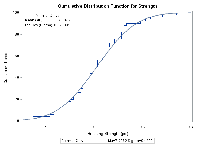
The plot shows a symmetric distribution with observations concentrated 6.9 and 7.1. The agreement between the empirical and the normal distribution functions in Output 4.35.1 is evidence that the normal distribution is an appropriate model for the distribution of breaking strengths.