The UNIVARIATE Procedure
- Overview
-
Getting Started

-
Syntax
-
Details
Missing Values Rounding Descriptive Statistics Calculating the Mode Calculating Percentiles Tests for Location Confidence Limits for Parameters of the Normal Distribution Robust Estimators Creating Line Printer Plots Creating High-Resolution Graphics Using the CLASS Statement to Create Comparative Plots Positioning Insets Formulas for Fitted Continuous Distributions Goodness-of-Fit Tests Kernel Density Estimates Construction of Quantile-Quantile and Probability Plots Interpretation of Quantile-Quantile and Probability Plots Distributions for Probability and Q-Q Plots Estimating Shape Parameters Using Q-Q Plots Estimating Location and Scale Parameters Using Q-Q Plots Estimating Percentiles Using Q-Q Plots Input Data Sets OUT= Output Data Set in the OUTPUT Statement OUTHISTOGRAM= Output Data Set OUTKERNEL= Output Data Set OUTTABLE= Output Data Set Tables for Summary Statistics ODS Table Names ODS Tables for Fitted Distributions ODS Graphics Computational Resources
-
Examples
Computing Descriptive Statistics for Multiple Variables Calculating Modes Identifying Extreme Observations and Extreme Values Creating a Frequency Table Creating Plots for Line Printer Output Analyzing a Data Set With a FREQ Variable Saving Summary Statistics in an OUT= Output Data Set Saving Percentiles in an Output Data Set Computing Confidence Limits for the Mean, Standard Deviation, and Variance Computing Confidence Limits for Quantiles and Percentiles Computing Robust Estimates Testing for Location Performing a Sign Test Using Paired Data Creating a Histogram Creating a One-Way Comparative Histogram Creating a Two-Way Comparative Histogram Adding Insets with Descriptive Statistics Binning a Histogram Adding a Normal Curve to a Histogram Adding Fitted Normal Curves to a Comparative Histogram Fitting a Beta Curve Fitting Lognormal, Weibull, and Gamma Curves Computing Kernel Density Estimates Fitting a Three-Parameter Lognormal Curve Annotating a Folded Normal Curve Creating Lognormal Probability Plots Creating a Histogram to Display Lognormal Fit Creating a Normal Quantile Plot Adding a Distribution Reference Line Interpreting a Normal Quantile Plot Estimating Three Parameters from Lognormal Quantile Plots Estimating Percentiles from Lognormal Quantile Plots Estimating Parameters from Lognormal Quantile Plots Comparing Weibull Quantile Plots Creating a Cumulative Distribution Plot Creating a P-P Plot
- References
| Kernel Density Estimates |
You can use the KERNEL option to superimpose kernel density estimates on histograms. Smoothing the data distribution with a kernel density estimate can be more effective than using a histogram to identify features that might be obscured by the choice of histogram bins or sampling variation. A kernel density estimate can also be more effective than a parametric curve fit when the process distribution is multi-modal. See Example 4.23.
The general form of the kernel density estimator is
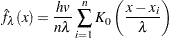 |
where
 is the kernel function
  is the bandwidth
  is the sample size
  is the
  th observation
  vertical scaling factor
and
 |
The KERNEL option provides three kernel functions ( ): normal, quadratic, and triangular. You can specify the function with the K= kernel-option in parentheses after the KERNEL option. Values for the K= option are NORMAL, QUADRATIC, and TRIANGULAR (with aliases of N, Q, and T, respectively). By default, a normal kernel is used. The formulas for the kernel functions are
 |
The value of , referred to as the bandwidth parameter, determines the degree of smoothness in the estimated density function. You specify indirectly by specifying a standardized bandwidth  with the C= kernel-option. If
  is the interquartile range and is the sample size, then is related to by the formula
 |
For a specific kernel function, the discrepancy between the density estimator  and the true density
  is measured by the mean integrated square error (MISE):
 |
The MISE is the sum of the integrated squared bias and the variance. An approximate mean integrated square error (AMISE) is:
 |
A bandwidth that minimizes AMISE can be derived by treating as the normal density that has parameters  and
and  estimated by the sample mean and standard deviation. If you do not specify a bandwidth parameter or if you specify C=MISE, the bandwidth that minimizes AMISE is used. The value of AMISE can be used to compare different density estimates. You can also specify C=SJPI to select the bandwidth by using a plug-in formula of Sheather and Jones (Jones, Marron, and Sheather; 1996). For each estimate, the bandwidth parameter , the kernel function type, and the value of AMISE are reported in the SAS log.
The general kernel density estimates assume that the domain of the density to estimate can take on all values on a real line. However, sometimes the domain of a density is an interval bounded on one or both sides. For example, if a variable Y is a measurement of only positive values, then the kernel density curve should be bounded so that is zero for negative Y values. You can use the LOWER= and UPPER= kernel-options to specify the bounds.
The UNIVARIATE procedure uses a reflection technique to create the bounded kernel density curve, as described in Silverman (1986, pp. 30-31). It adds the reflections of the kernel density that are outside the boundary to the bounded kernel estimates. The general form of the bounded kernel density estimator is computed by replacing  in the original equation with
 |
where  is the lower bound and
  is the upper bound.
Without a lower bound,  and
and 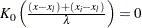 . Similarly, without an upper bound,
  and
and  .
.
When C=MISE is used with a bounded kernel density, the UNIVARIATE procedure uses a bandwidth that minimizes the AMISE for its corresponding unbounded kernel.