The UNIVARIATE Procedure
- Overview
-
Getting Started

-
Syntax

-
Details
 Missing Values Rounding Descriptive Statistics Calculating the Mode Calculating Percentiles Tests for Location Confidence Limits for Parameters of the Normal Distribution Robust Estimators Creating Line Printer Plots Creating High-Resolution Graphics Using the CLASS Statement to Create Comparative Plots Positioning Insets Formulas for Fitted Continuous Distributions Goodness-of-Fit Tests Kernel Density Estimates Construction of Quantile-Quantile and Probability Plots Interpretation of Quantile-Quantile and Probability Plots Distributions for Probability and Q-Q Plots Estimating Shape Parameters Using Q-Q Plots Estimating Location and Scale Parameters Using Q-Q Plots Estimating Percentiles Using Q-Q Plots Input Data Sets OUT= Output Data Set in the OUTPUT Statement OUTHISTOGRAM= Output Data Set OUTKERNEL= Output Data Set OUTTABLE= Output Data Set Tables for Summary Statistics ODS Table Names ODS Tables for Fitted Distributions ODS Graphics Computational Resources
 -
Examples
 Computing Descriptive Statistics for Multiple Variables Calculating Modes Identifying Extreme Observations and Extreme Values Creating a Frequency Table Creating Plots for Line Printer Output Analyzing a Data Set With a FREQ Variable Saving Summary Statistics in an OUT= Output Data Set Saving Percentiles in an Output Data Set Computing Confidence Limits for the Mean, Standard Deviation, and Variance Computing Confidence Limits for Quantiles and Percentiles Computing Robust Estimates Testing for Location Performing a Sign Test Using Paired Data Creating a Histogram Creating a One-Way Comparative Histogram Creating a Two-Way Comparative Histogram Adding Insets with Descriptive Statistics Binning a Histogram Adding a Normal Curve to a Histogram Adding Fitted Normal Curves to a Comparative Histogram Fitting a Beta Curve Fitting Lognormal, Weibull, and Gamma Curves Computing Kernel Density Estimates Fitting a Three-Parameter Lognormal Curve Annotating a Folded Normal Curve Creating Lognormal Probability Plots Creating a Histogram to Display Lognormal Fit Creating a Normal Quantile Plot Adding a Distribution Reference Line Interpreting a Normal Quantile Plot Estimating Three Parameters from Lognormal Quantile Plots Estimating Percentiles from Lognormal Quantile Plots Estimating Parameters from Lognormal Quantile Plots Comparing Weibull Quantile Plots Creating a Cumulative Distribution Plot Creating a P-P Plot
 - References
| Exploring a Data Distribution |
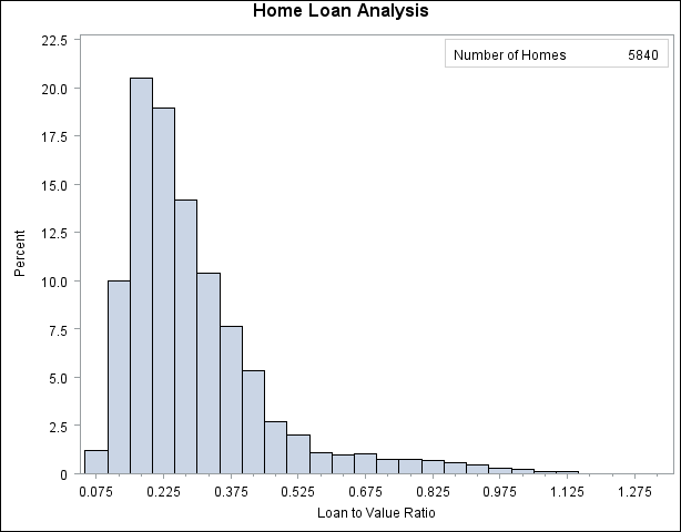
Figure 4.2 shows a histogram of the loan-to-value ratios. The histogram reveals features of the ratio distribution, such as its skewness and the peak at 0.175, which are not evident from the tables in the previous example. The following statements create the histogram:
ods graphics off;
title 'Home Loan Analysis';
proc univariate data=HomeLoans noprint;
   histogram LoanToValueRatio;
   inset n = 'Number of Homes' / position=ne;
run;
By default, PROC UNIVARIATE produces traditional graphics output, and the basic appearance of the histogram is determined by the prevailing ODS style. The NOPRINT option suppresses the display of summary statistics. The INSET statement inserts the total number of analyzed home loans in the upper right (northeast) corner of the plot.

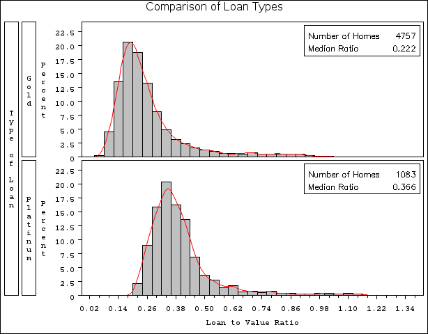
The data set HomeLoans contains a variable named LoanType that classifies the loans into two types: Gold and Platinum. It is useful to compare the distributions of LoanToValueRatio for the two types. The following statements request quantiles for each distribution and a comparative histogram, which are shown in Figure 4.3 and Figure 4.4.
title 'Comparison of Loan Types';
options nogstyle;
ods select Quantiles MyHist;
proc univariate data=HomeLoans;
   var LoanToValueRatio;
   class LoanType;
   histogram LoanToValueRatio / kernel(color=red)
                                cfill=ltgray
                                name='MyHist';
   inset n='Number of Homes' median='Median Ratio' (5.3) / position=ne;
   label LoanType = 'Type of Loan';
run;
options gstyle;
The ODS SELECT statement restricts the default output to the tables of quantiles and the graph produced by the HISTOGRAM statement, which is identified by the value specified by the NAME= option. The CLASS statement specifies LoanType as a classification variable for the quantile computations and comparative histogram. The KERNEL option adds a smooth nonparametric estimate of the ratio density to each histogram. The INSET statement specifies summary statistics to be displayed directly in the graph.
The NOGSTYLE system option specifies that the ODS style not influence the appearance of the histogram. Instead, the CFILL= option determines the color of the histogram bars and the COLOR= option specifies the color of the kernel density curve.
| Comparison of Loan Types |
| Quantiles (Definition 5) | |
|---|---|
| Quantile | Estimate |
| 100% Max | 1.0617647 |
| 99% | 0.8974576 |
| 95% | 0.6385908 |
| 90% | 0.4471369 |
| 75% Q3 | 0.2985099 |
| 50% Median | 0.2217033 |
| 25% Q1 | 0.1734568 |
| 10% | 0.1411130 |
| 5% | 0.1213079 |
| 1% | 0.0942167 |
| 0% Min | 0.0651786 |
| Comparison of Loan Types |
| Quantiles (Definition 5) | |
|---|---|
| Quantile | Estimate |
| 100% Max | 1.312981 |
| 99% | 1.050000 |
| 95% | 0.691803 |
| 90% | 0.549273 |
| 75% Q3 | 0.430160 |
| 50% Median | 0.366168 |
| 25% Q1 | 0.314452 |
| 10% | 0.273670 |
| 5% | 0.253124 |
| 1% | 0.231114 |
| 0% Min | 0.215504 |
The output in Figure 4.3 shows that the median ratio for Platinum loans (0.366) is greater than the median ratio for Gold loans (0.222). The comparative histogram in Figure 4.4 enables you to compare the two distributions more easily. It shows that the ratio distributions are similar except for a shift of about 0.14.

A sample program for this example, univar1.sas, is available in the SAS Sample Library for Base SAS software.