The UNIVARIATE Procedure

CDFPLOT Statement

CDFPLOT <variables> < / options> ;

The CDFPLOT statement plots the observed cumulative distribution function (cdf) of a variable, defined as

	$\text{[math]}$	$\text{[math]}$	$\text{[math]}$
	$\text{[math]}$	$\text{[math]}$	$\text{[math]}$

where $\text{[math]}$ is the number of nonmissing observations. The cdf is an increasing step function that has a vertical jump of $\text{[math]}$ at each value of $\text{[math]}$ equal to an observed value. The cdf is also referred to as the empirical cumulative distribution function (ecdf).

You can use any number of CDFPLOT statements in the UNIVARIATE procedure. The components of the CDFPLOT statement are as follows.

variables

specify variables for which to create cdf plots. If you specify a VAR statement, the variables must also be listed in the VAR statement. Otherwise, the variables can be any numeric variables in the input data set. If you do not specify a list of variables, then by default the procedure creates a cdf plot for each variable listed in the VAR statement, or for each numeric variable in the DATA= data set if you do not specify a VAR statement.

For example, suppose a data set named Steel contains exactly three numeric variables: Length, Width, and Height. The following statements create a cdf plot for each of the three variables:

proc univariate data=Steel;
   cdfplot;
run;

The following statements create a cdf plot for Length and a cdf plot for Width:

proc univariate data=Steel;
   var Length Width;
   cdfplot;
run;

The following statements create a cdf plot for Width:

proc univariate data=Steel;
   var Length Width;
   cdfplot Width;
run;

options

specify the theoretical distribution for the plot or add features to the plot. If you specify more than one variable, the options apply equally to each variable. Specify all options after the slash (/) in the CDFPLOT statement. You can specify only one option that names a distribution in each CDFPLOT statement, but you can specify any number of other options. The distributions available are listed in Table 4.2. By default, the procedure produces a plot for the normal distribution.

Table 4.2 through Table 4.15 list the CDFPLOT options by function. For complete descriptions, see the sections Dictionary of Options and Dictionary of Common Options. Options can be any of the following:

primary options
secondary options
general options

Distribution Options

Table 4.2 lists primary options for requesting a theoretical distribution.

Table 4.2 Primary Options for Theoretical Distributions
Option	Description
BETA(beta-options)	plots two-parameter beta distribution function, parameters $\text{[math]}$ and $\text{[math]}$ assumed known
EXPONENTIAL(exponential-options)	plots one-parameter exponential distribution function, parameter $\text{[math]}$ assumed known
GAMMA(gamma-options)	plots two-parameter gamma distribution function, parameter $\text{[math]}$ assumed known
GUMBEL(Gumbel-options)	plots Gumbel distribution with location parameter $\text{[math]}$ and scale parameter $\text{[math]}$
IGAUSS(iGauss-options)	plots inverse Gaussian distribution with mean $\text{[math]}$ and shape parameter $\text{[math]}$
LOGNORMAL(lognormal-options)	plots two-parameter lognormal distribution function, parameter $\text{[math]}$ assumed known
NORMAL(normal-options)	plots normal distribution function
PARETO(Pareto-options)	plots generalized Pareto distribution with threshold parameter $\text{[math]}$ , scale parameter $\text{[math]}$ , and shape parameter $\text{[math]}$
POWER(power-options)	plots power function distribution with threshold parameter $\text{[math]}$ , scale parameter $\text{[math]}$ , and shape parameter $\text{[math]}$
RAYLEIGH(Rayleigh-options)	plots Rayleigh distribution with threshold parameter $\text{[math]}$ and scale parameter $\text{[math]}$
WEIBULL(Weibull-options)	plots two-parameter Weibull distribution function, parameter $\text{[math]}$ assumed known

Table 4.3 through Table 4.14 list secondary options that specify distribution parameters and control the display of a theoretical distribution function. Specify these options in parentheses after the distribution keyword. For example, you can request a normal probability plot with a distribution reference line by specifying the NORMAL option as follows:

proc univariate;
   cdfplot / normal(mu=10 sigma=0.5 color=red);
run;

The COLOR= option specifies the color for the curve, and the normal-options MU= and SIGMA= specify the parameters $\text{[math]}$ and $\text{[math]}$ for the distribution function. If you do not specify these parameters, maximum likelihood estimates are computed.

Table 4.3 Secondary Options Used with All Distributions
Option	Description
COLOR=	specifies color of theoretical distribution function
L=	specifies line type of theoretical distribution function
W=	specifies width of theoretical distribution function

Table 4.4 Secondary Beta-Options
Option	Description
ALPHA=	specifies first shape parameter $\text{[math]}$ for beta distribution function
BETA=	specifies second shape parameter $\text{[math]}$ for beta distribution function
SIGMA=	specifies scale parameter $\text{[math]}$ for beta distribution function
THETA=	specifies lower threshold parameter $\text{[math]}$ for beta distribution function

Table 4.5 Secondary Exponential-Options
Option	Description
SIGMA=	specifies scale parameter $\text{[math]}$ for exponential distribution function
THETA=	specifies threshold parameter $\text{[math]}$ for exponential distribution function

Table 4.6 Secondary Gamma-Options
Option	Description
ALPHA=	specifies shape parameter $\text{[math]}$ for gamma distribution function
ALPHADELTA=	specifies change in successive estimates of $\text{[math]}$ at which the Newton-Raphson approximation of $\text{[math]}$ terminates
ALPHAINITIAL=	specifies initial value for $\text{[math]}$ in the Newton-Raphson approximation of $\text{[math]}$
MAXITER=	specifies maximum number of iterations in the Newton-Raphson approximation of $\text{[math]}$
SIGMA=	specifies scale parameter $\text{[math]}$ for gamma distribution function
THETA=	specifies threshold parameter $\text{[math]}$ for gamma distribution function

Table 4.7 Secondary Gumbel-Options
Option	Description
MU=	specifies location parameter $\text{[math]}$ for Gumbel distribution function
SIGMA=	specifies scale parameter $\text{[math]}$ for Gumbel distribution function

Table 4.8 Secondary IGauss-Options
Option	Description
LAMBDA=	specifies shape parameter $\text{[math]}$ for inverse Gaussian distribution function
MU=	specifies mean $\text{[math]}$ for inverse Gaussian distribution function

Table 4.9 Secondary Lognormal-Options
Option	Description
SIGMA=	specifies shape parameter $\text{[math]}$ for lognormal distribution function
THETA=	specifies threshold parameter $\text{[math]}$ for lognormal distribution function
ZETA=	specifies scale parameter $\text{[math]}$ for lognormal distribution function

Table 4.10 Secondary Normal-Options
Option	Description
MU=	specifies mean $\text{[math]}$ for normal distribution function
SIGMA=	specifies standard deviation $\text{[math]}$ for normal distribution function

Table 4.11 Secondary Pareto-Options
Option	Description
ALPHA=	specifies shape parameter $\text{[math]}$ for generalized Pareto distribution function
SIGMA=	specifies scale parameter $\text{[math]}$ for generalized Pareto distribution function
THETA=	specifies threshold parameter $\text{[math]}$ for generalized Pareto distribution function

Table 4.12 Secondary Power-Options
Option	Description
ALPHA=	specifies shape parameter $\text{[math]}$ for power function distribution
SIGMA=	specifies scale parameter $\text{[math]}$ for power function distribution
THETA=	specifies threshold parameter $\text{[math]}$ for power function distribution

Table 4.13 Secondary Rayleigh-Options
Option	Description
SIGMA=	specifies scale parameter $\text{[math]}$ for Rayleigh distribution function
THETA=	specifies threshold parameter $\text{[math]}$ for Rayleigh distribution function

Table 4.14 Secondary Weibull-Options
Option	Description
C=	specifies shape parameter $\text{[math]}$ for Weibull distribution function
CDELTA=	specifies change in successive estimates of $\text{[math]}$ at which the Newton-Raphson approximation of $\text{[math]}$ terminates
CINITIAL=	specifies initial value for $\text{[math]}$ in the Newton-Raphson approximation of $\text{[math]}$
MAXITER=	specifies maximum number of iterations in the Newton-Raphson approximation of $\text{[math]}$
SIGMA=	specifies scale parameter $\text{[math]}$ for Weibull distribution function
THETA=	specifies threshold parameter $\text{[math]}$ for Weibull distribution function

General Options

Table 4.15 summarizes general options for enhancing cdf plots.

Table 4.15 General Graphics Options
Option	Description
ANNOKEY	applies annotation requested in ANNOTATE= data set to key cell only
ANNOTATE=	specifies annotate data set
CAXIS=	specifies color for axis
CFRAME=	specifies color for frame
CFRAMESIDE=	specifies color for filling row label frames
CFRAMETOP=	specifies color for filling column label frames
CHREF=	specifies color for HREF= lines
CONTENTS=	specifies table of contents entry for cdf plot grouping
CPROP=	specifies color for proportion of frequency bar
CTEXT=	specifies color for text
CTEXTSIDE=	specifies color for row labels
CTEXTTOP=	specifies color for column labels
CVREF=	specifies color for VREF= lines
DESCRIPTION=	specifies description for graphics catalog member
FONT=	specifies text font
HAXIS=	specifies AXIS statement for horizontal axis
HEIGHT=	specifies height of text used outside framed areas
HMINOR=	specifies number of horizontal axis minor tick marks
HREF=	specifies reference lines perpendicular to the horizontal axis
HREFLABELS=	specifies labels for HREF= lines
HREFLABPOS=	specifies position for HREF= line labels
INFONT=	specifies software font for text inside framed areas
INHEIGHT=	specifies height of text inside framed areas
INTERTILE=	specifies distance between tiles in comparative plot
LHREF=	specifies line style for HREF= lines
LVREF=	specifies line style for VREF= lines
NAME=	specifies name for plot in graphics catalog
NCOLS=	specifies number of columns in comparative plot
NOECDF	suppresses plot of empirical (observed) distribution function
NOFRAME	suppresses frame around plotting area
NOHLABEL	suppresses label for horizontal axis
NOVLABEL	suppresses label for vertical axis
NOVTICK	suppresses tick marks and tick mark labels for vertical axis
NROWS=	specifies number of rows in comparative plot
OVERLAY	overlays plots for different class levels (ODS Graphics only)
TURNVLABELS	turns and vertically strings out characters in labels for vertical axis
VAXIS=	specifies AXIS statement for vertical axis
VAXISLABEL=	specifies label for vertical axis
VMINOR=	specifies number of vertical axis minor tick marks
VREF=	specifies reference lines perpendicular to the vertical axis
VREFLABELS=	specifies labels for VREF= lines
VREFLABPOS=	specifies position for VREF= line labels
VSCALE=	specifies scale for vertical axis
WAXIS=	specifies line thickness for axes and frame

Dictionary of Options

The following entries provide detailed descriptions of the options specific to the CDFPLOT statement. See the section Dictionary of Common Options for detailed descriptions of options common to all plot statements.

ALPHA=value

specifies the shape parameter $\text{[math]}$ for distribution functions requested with the BETA, GAMMA, PARETO, and POWER options. Enclose the ALPHA= option in parentheses after the distribution keyword. If you do not specify a value for $\text{[math]}$ , the procedure calculates a maximum likelihood estimate. For examples, see the entries for the BETA and GAMMA options.

BETA<(beta-options )>

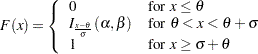
displays a fitted beta distribution function on the cdf plot. The equation of the fitted cdf is

$\text{[math]}$

where $\text{[math]}$ is the incomplete beta function and

$\text{[math]}$ lower threshold parameter (lower endpoint)
$\text{[math]}$ scale parameter $\text{[math]}$
$\text{[math]}$ shape parameter $\text{[math]}$
$\text{[math]}$ shape parameter $\text{[math]}$

The beta distribution is bounded below by the parameter $\text{[math]}$ and above by the value $\text{[math]}$ . You can specify $\text{[math]}$ and $\text{[math]}$ by using the THETA= and SIGMA= beta-options, as illustrated in the following statements, which fit a beta distribution bounded between 50 and 75. The default values for $\text{[math]}$ and $\text{[math]}$ are 0 and 1, respectively.

proc univariate;
   cdfplot / beta(theta=50 sigma=25);
run;

The beta distribution has two shape parameters: $\text{[math]}$ and $\text{[math]}$ . If these parameters are known, you can specify their values with the ALPHA= and BETA= beta-options. If you do not specify values for $\text{[math]}$ and $\text{[math]}$ , the procedure calculates maximum likelihood estimates.

The BETA option can appear only once in a CDFPLOT statement. Table 4.3 and Table 4.4 list options you can specify with the BETA distribution option.

BETA=value

B=value

specifies the second shape parameter $\text{[math]}$ for beta distribution functions requested by the BETA option. Enclose the BETA= option in parentheses after the BETA keyword. If you do not specify a value for $\text{[math]}$ , the procedure calculates a maximum likelihood estimate. For examples, see the preceding entry for the BETA option.

C=value

specifies the shape parameter $\text{[math]}$ for Weibull distribution functions requested with the WEIBULL option. Enclose the C= option in parentheses after the WEIBULL keyword. If you do not specify a value for $\text{[math]}$ , the procedure calculates a maximum likelihood estimate. You can specify the SHAPE= option as an alias for the C= option.

EXPONENTIAL<(exponential-options )>

EXP<(exponential-options )>

displays a fitted exponential distribution function on the cdf plot. The equation of the fitted cdf is

$\text{[math]}$

where

$\text{[math]}$ threshold parameter
$\text{[math]}$ scale parameter $\text{[math]}$

The parameter $\text{[math]}$ must be less than or equal to the minimum data value. You can specify $\text{[math]}$ with the THETA= exponential-option. The default value for $\text{[math]}$ is 0. You can specify $\text{[math]}$ with the SIGMA= exponential-option. By default, a maximum likelihood estimate is computed for $\text{[math]}$ . For example, the following statements fit an exponential distribution with $\text{[math]}$ and a maximum likelihood estimate for $\text{[math]}$ :

proc univariate;
   cdfplot / exponential(theta=10 l=2 color=green);
run;

The exponential curve is green and has a line type of 2.

The EXPONENTIAL option can appear only once in a CDFPLOT statement. Table 4.3 and Table 4.5 list the options you can specify with the EXPONENTIAL option.

GAMMA<(gamma-options)>

displays a fitted gamma distribution function on the cdf plot. The equation of the fitted cdf is

$\text{[math]}$

where

$\text{[math]}$ threshold parameter
$\text{[math]}$ scale parameter $\text{[math]}$
$\text{[math]}$ shape parameter $\text{[math]}$

The parameter $\text{[math]}$ for the gamma distribution must be less than the minimum data value. You can specify $\text{[math]}$ with the THETA= gamma-option. The default value for $\text{[math]}$ is 0. In addition, the gamma distribution has a shape parameter $\text{[math]}$ and a scale parameter $\text{[math]}$ . You can specify these parameters with the ALPHA= and SIGMA= gamma-options. By default, maximum likelihood estimates are computed for $\text{[math]}$ and $\text{[math]}$ . For example, the following statements fit a gamma distribution function with $\text{[math]}$ and maximum likelihood estimates for $\text{[math]}$ and $\text{[math]}$ :

proc univariate;
   cdfplot / gamma(theta=4);
run;

Note that the maximum likelihood estimate of $\text{[math]}$ is calculated iteratively using the Newton-Raphson approximation. The gamma-options ALPHADELTA=, ALPHAINITIAL=, and MAXITER= control the approximation.

The GAMMA option can appear only once in a CDFPLOT statement. Table 4.3 and Table 4.6 list the options you can specify with the GAMMA option.

GUMBEL<(Gumbel-options)>

displays a fitted Gumbel distribution (also known as Type 1 extreme value distribution) function on the cdf plot. The equation of the fitted cdf is

$\text{[math]}$

where

$\text{[math]}$ location parameter
$\text{[math]}$ scale parameter $\text{[math]}$

You can specify known values for $\text{[math]}$ and $\text{[math]}$ with the MU= and SIGMA= Gumbel-options. By default, maximum likelihood estimates are computed for $\text{[math]}$ and $\text{[math]}$ .

The GUMBEL option can appear only once in a CDFPLOT statement. Table 4.3 and Table 4.7 list secondary options you can specify with the GUMBEL option.

IGAUSS<(iGauss-options)>

displays a fitted inverse Gaussian distribution function on the cdf plot. The equation of the fitted cdf is

$\text{[math]}$

where $\text{[math]}$ is the standard normal cumulative distribution function, and

$\text{[math]}$ mean parameter $\text{[math]}$
$\text{[math]}$ shape parameter $\text{[math]}$

You can specify known values for $\text{[math]}$ and $\text{[math]}$ with the MU= and LAMBDA= iGauss-options. By default, maximum likelihood estimates are computed for $\text{[math]}$ and $\text{[math]}$ .

The IGAUSS option can appear only once in a CDFPLOT statement. Table 4.3 and Table 4.8 list secondary options you can specify with the IGAUSS option.

LAMBDA=value

specifies the shape parameter $\text{[math]}$ for distribution functions requested with the IGAUSS option. Enclose the LAMBDA= option in parentheses after the IGAUSS distribution keyword. If you do not specify a value for $\text{[math]}$ , the procedure calculates a maximum likelihood estimate.

LOGNORMAL<(lognormal-options)>

displays a fitted lognormal distribution function on the cdf plot. The equation of the fitted cdf is

$\text{[math]}$

where $\text{[math]}$ is the standard normal cumulative distribution function and

$\text{[math]}$ threshold parameter
$\text{[math]}$ scale parameter
$\text{[math]}$ shape parameter $\text{[math]}$

The parameter $\text{[math]}$ for the lognormal distribution must be less than the minimum data value. You can specify $\text{[math]}$ with the THETA= lognormal-option. The default value for $\text{[math]}$ is 0. In addition, the lognormal distribution has a shape parameter $\text{[math]}$ and a scale parameter $\text{[math]}$ . You can specify these parameters with the SIGMA= and ZETA= lognormal-options. By default, maximum likelihood estimates are computed for $\text{[math]}$ and $\text{[math]}$ . For example, the following statements fit a lognormal distribution function with $\text{[math]}$ and maximum likelihood estimates for $\text{[math]}$ and $\text{[math]}$ :

proc univariate;
   cdfplot / lognormal(theta = 10);
run;

The LOGNORMAL option can appear only once in a CDFPLOT statement. Table 4.3 and Table 4.9 list options that you can specify with the LOGNORMAL option.

MU=value

specifies the parameter $\text{[math]}$ for theoretical cumulative distribution functions requested with the GUMBEL, IGAUSS, and NORMAL option. Enclose the MU= option in parentheses after the distribution keyword. For the inverse Gaussian and normal distributions, the default value is the sample mean. If you do not specify a value for $\text{[math]}$ for the Gumbel distribution, the procedure calculates a maximum likelihood estimate. For an example, see the entry for the NORMAL option.

NOECDF

suppresses the observed distribution function (the empirical cumulative distribution function) of the variable, which is drawn by default. This option enables you to create theoretical cdf plots without displaying the data distribution. The NOECDF option can be used only with a theoretical distribution (such as the NORMAL option).

NORMAL<(normal-options)>

displays a fitted normal distribution function on the cdf plot. The equation of the fitted cdf is

$\text{[math]}$

where $\text{[math]}$ is the standard normal cumulative distribution function and

$\text{[math]}$ mean
$\text{[math]}$ standard deviation $\text{[math]}$

You can specify known values for $\text{[math]}$ and $\text{[math]}$ with the MU= and SIGMA= normal-options, as shown in the following statements:

proc univariate;
   cdfplot / normal(mu=14 sigma=.05);
run;

By default, the sample mean and sample standard deviation are calculated for $\text{[math]}$ and $\text{[math]}$ . The NORMAL option can appear only once in a CDFPLOT statement. Table 4.3 and Table 4.10 list options that you can specify with the NORMAL option.

PARETO<(Pareto-options)>

displays a fitted generalized Pareto distribution function on the cdf plot. The equation of the fitted cdf is

$\text{[math]}$

where

$\text{[math]}$ threshold parameter
$\text{[math]}$ scale parameter $\text{[math]}$
$\text{[math]}$ shape parameter

The parameter $\text{[math]}$ for the generalized Pareto distribution must be less than the minimum data value. You can specify $\text{[math]}$ with the THETA= Pareto-option. The default value for $\text{[math]}$ is 0. In addition, the generalized Pareto distribution has a shape parameter $\text{[math]}$ and a scale parameter $\text{[math]}$ . You can specify these parameters with the ALPHA= and SIGMA= Pareto-options. By default, maximum likelihood estimates are computed for $\text{[math]}$ and $\text{[math]}$ .

The PARETO option can appear only once in a CDFPLOT statement. Table 4.3 and Table 4.11 list options that you can specify with the PARETO option.

POWER<(power-options)>

displays a fitted power function distribution on the cdf plot. The equation of the fitted cdf is

$\text{[math]}$

where

$\text{[math]}$ lower threshold parameter (lower endpoint)
$\text{[math]}$ scale parameter $\text{[math]}$
$\text{[math]}$ shape parameter $\text{[math]}$

The power function distribution is bounded below by the parameter $\text{[math]}$ and above by the value $\text{[math]}$ . You can specify $\text{[math]}$ and $\text{[math]}$ by using the THETA= and SIGMA= power-options. The default values for $\text{[math]}$ and $\text{[math]}$ are 0 and 1, respectively.

You can specify a value for the shape parameter, $\text{[math]}$ , with the ALPHA= power-option. If you do not specify a value for $\text{[math]}$ , the procedure calculates a maximum likelihood estimate.

The power function distribution is a special case of the beta distribution with its second shape parameter, $\text{[math]}$ .

The POWER option can appear only once in a CDFPLOT statement. Table 4.3 and Table 4.12 list options that you can specify with the POWER option.

RAYLEIGH<(Rayleigh-options)>

displays a fitted Rayleigh distribution function on the cdf plot. The equation of the fitted cdf is

$\text{[math]}$

where

$\text{[math]}$ threshold parameter
$\text{[math]}$ scale parameter $\text{[math]}$

The parameter $\text{[math]}$ for the Rayleigh distribution must be less than the minimum data value. You can specify $\text{[math]}$ with the THETA= Rayleigh-option. The default value for $\text{[math]}$ is 0. You can specify $\text{[math]}$ with the SIGMA= Rayleigh-option. By default, a maximum likelihood estimate is computed for $\text{[math]}$ .

The RAYLEIGH option can appear only once in a CDFPLOT statement. Table 4.3 and Table 4.13 list options that you can specify with the RAYLEIGH option.

SIGMA=value | EST

specifies the parameter $\text{[math]}$ for distribution functions requested by the BETA, EXPONENTIAL, GAMMA, LOGNORMAL, NORMAL, and WEIBULL options. Enclose the SIGMA= option in parentheses after the distribution keyword. The following table summarizes the use of the SIGMA= option:

Distribution Option	SIGMA= Specifies	Default Value	Alias
BETA	scale parameter $\text{[math]}$	1	SCALE=
EXPONENTIAL	scale parameter $\text{[math]}$	maximum likelihood estimate	SCALE=
GAMMA	scale parameter $\text{[math]}$	maximum likelihood estimate	SCALE=
GUMBEL	scale parameter $\text{[math]}$	maximum likelihood estimate
LOGNORMAL	shape parameter $\text{[math]}$	maximum likelihood estimate	SHAPE=
NORMAL	scale parameter $\text{[math]}$	standard deviation
PARETO	scale parameter $\text{[math]}$	maximum likelihood estimate
POWER	scale parameter $\text{[math]}$	1
RAYLEIGH	scale parameter $\text{[math]}$	maximum likelihood estimate
WEIBULL	scale parameter $\text{[math]}$	maximum likelihood estimate	SCALE=

THETA=value | EST

THRESHOLD=value | EST

specifies the lower threshold parameter $\text{[math]}$ for theoretical cumulative distribution functions requested with the BETA, EXPONENTIAL, GAMMA, LOGNORMAL, PARETO, POWER, RAYLEIGH, and WEIBULL options. Enclose the THETA= option in parentheses after the distribution keyword. The default value is 0.

VSCALE=PERCENT | PROPORTION

specifies the scale of the vertical axis. The value PERCENT scales the data in units of percent of observations per data unit. The value PROPORTION scales the data in units of proportion of observations per data unit. The default is PERCENT.

WEIBULL<(Weibull-options)>

displays a fitted Weibull distribution function on the cdf plot. The equation of the fitted cdf is

$\text{[math]}$

where

$\text{[math]}$ threshold parameter
$\text{[math]}$ scale parameter $\text{[math]}$
$\text{[math]}$ shape parameter $\text{[math]}$

The parameter $\text{[math]}$ must be less than the minimum data value. You can specify $\text{[math]}$ with the THETA= Weibull-option. The default value for $\text{[math]}$ is 0. In addition, the Weibull distribution has a shape parameter $\text{[math]}$ and a scale parameter $\text{[math]}$ . You can specify these parameters with the SIGMA= and C= Weibull-options. By default, maximum likelihood estimates are computed for $\text{[math]}$ and $\text{[math]}$ . For example, the following statements fit a Weibull distribution function with $\text{[math]}$ and maximum likelihood estimates for $\text{[math]}$ and $\text{[math]}$ :

proc univariate;
   cdfplot / weibull(theta=15);
run;

Note that the maximum likelihood estimate of $\text{[math]}$ is calculated iteratively using the Newton-Raphson approximation. The Weibull-options CDELTA=, CINITIAL=, and MAXITER= control the approximation.

The WEIBULL option can appear only once in a CDFPLOT statement. Table 4.3 and Table 4.14 list options that you can specify with the WEIBULL option.

ZETA=value

specifies a value for the scale parameter $\text{[math]}$ for a lognormal distribution function requested with the LOGNORMAL option. Enclose the ZETA= option in parentheses after the LOGNORMAL keyword. If you do not specify a value for $\text{[math]}$ , a maximum likelihood estimate is computed. You can specify the SCALE= option as an alias for the ZETA= option.