The VARMAX Procedure
- Overview
-
Getting Started

-
Syntax
-
DetailsMissing ValuesVARMAX ModelDynamic Simultaneous Equations ModelingImpulse Response FunctionForecastingTentative Order SelectionVAR and VARX ModelingBayesian VAR and VARX ModelingVARMA and VARMAX ModelingModel Diagnostic ChecksCointegrationVector Error Correction ModelingI(2) ModelMultivariate GARCH ModelingOutput Data SetsOUT= Data SetOUTEST= Data SetOUTHT= Data SetOUTSTAT= Data SetPrinted OutputODS Table NamesODS GraphicsComputational Issues
-
Examples
- References
The MODEL statement specifies dependent (endogenous) variables and independent (exogenous) variables for the VARMAX model. The multivariate model can have the same or different independent variables corresponding to the dependent variables. As a special case, the VARMAX procedure allows you to analyze one dependent variable. Only one MODEL statement is allowed.
For example, the following statements are equivalent ways of specifying the multivariate model for the vector ![]() :
:
   model y1 y2 y3 </options>;
   model y1-y3 </options>;
The following statements are equivalent ways of specifying the multivariate model with independent variables, where ![]() , and
, and ![]() are the dependent variables and
are the dependent variables and ![]() , and
, and ![]() are the independent variables:
are the independent variables:
   model y1 y2 y3 y4 = x1 x2 x3 x4 x5 </options>;
   model y1 y2 y3 y4 = x1-x5 </options>;
   model y1 = x1-x5, y2 = x1-x5, y3 y4 = x1-x5 </options>;
   model y1-y4 = x1-x5 </options>;
When the multivariate model has different independent variables that correspond to each of the dependent variables, equations are separated by commas (,) and the model can be specified as illustrated by the following MODEL statement:
model y1 = x1-x3, y2 = x3-x5, y3 y4 = x1-x5 </options>;
The following options can be used in the MODEL statement after a forward slash (/):
- CENTER
-
centers the dependent (endogenous) variables by subtracting their means. Note that centering is done after differencing when the DIF= or DIFY= option is specified. If there are exogenous (independent) variables, this option is not applicable.
model y1 y2 / p=1 center;
-
DIF(variable (number-list) <... variable (number-list)>)
DIF=(variable (number-list) <... variable (number-list)>) -
specifies the degrees of differencing to be applied to the specified dependent or independent variables. The number-list must contain one or more numbers, each of which should be greater than zero. The differencing can be the same for all variables, or it can vary among variables. For example, the DIF=(
 (1,4)
(1,4)  (1)
(1)  (2)) option specifies that the series is differenced at lag 1 and at lag 4, which is
![\[ (1-B^4)(1-B)y_{1t}=(y_{1t}-y_{1,t-1})-(y_{1,t-4}-y_{1,t-5}) \]](images/etsug_varmax0113.png)
the series
is differenced at lag 1, which is  ; and the series is differenced at lag 2, which is
  .
.
The following uses the data
 ,
,  ,
,  , and
, and  , where
  and
and  .
.
model y1 y2 = x1 x2 / p=1 dif=(y1(1) x2(2));
-
DIFX(number-list)
DIFX=(number-list) -
specifies the degrees of differencing to be applied to all independent variables. The number-list must contain one or more numbers, each of which should be greater than zero. For example, the DIFX=(1) option specifies that all of the independent series are differenced once at lag 1. The DIFX=(1,4) option specifies that all of the independent series are differenced at lag 1 and at lag 4. If independent variables are specified in the DIF= option, then the DIFX= option is ignored.
The following statement uses the data
 , ,
, ,  , and , where
  and
and  .
.
model y1 y2 = x1 x2 / p=1 difx(1);
-
DIFY(number-list)
DIFY=(number-list) -
specifies the degrees of differencing to be applied to all dependent (endogenous) variables. The number-list must contain one or more numbers, each of which should be greater than zero. For details, see the DIFX= option. If dependent variables are specified in the DIF= option, then the DIFY= option is ignored.
model y1 y2 / p=1 dify(1);
- METHOD=value
-
requests the type of estimates to be computed. The possible values of the METHOD= option are as follows:
- LS
-
specifies least squares estimates.
- ML
-
specifies maximum likelihood estimates.
When the ECM=, PRIOR=, and Q= options and the GARCH statement are specified, the default ML method is used regardless of the method given by the METHOD= option.
model y1 y2 / p=1 method=ml;
- NOCURRENTX
-
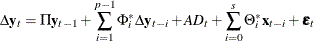
suppresses the current values
 of the independent variables. In general, the VARX(
 ) model is
![\[ \mb{y} _ t = \bdelta + \sum _{i=1}^{p}\Phi _ i\mb{y} _{t-i} + \sum _{i=0}^{s}\Theta _ i^*\mb{x} _{t-i} + \bepsilon _ t \]](images/etsug_varmax0125.png)
where p is the number of lags of the dependent variables included in the model, and s is the number of lags of the independent variables included in the model, including the contemporaneous values of
.
A VARX(1,2) model can be specified as:
model y1 y2 = x1 x2 / p=1 xlag=2;
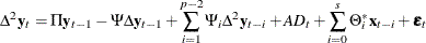
If the NOCURRENTX option is specified, it suppresses the current values
 and starts with
  . The VARX() model is redefined as:
![\[ \mb{y} _ t = \bdelta + \sum _{i=1}^{p}\Phi _ i\mb{y} _{t-i} + \sum _{i=1}^{s}\Theta _ i^*\mb{x} _{t-i} + \bepsilon _ t \]](images/etsug_varmax0128.png)
This model with
 and
and  can be specified as:
model y1 y2 = x1 x2 / p=1 xlag=2 nocurrentx;
- NOINT
-
suppresses the intercept parameter
 .
.
model y1 y2 / p=1 noint;
- NSEASON=number
-
specifies the number of seasonal periods. When the NSEASON=number option is specified, (number –1) seasonal dummies are added to the regressors. If the NOINT option is specified, the NSEASON= option is not applicable.
model y1 y2 / p=1 nseason=4;
- SCENTER
-
centers seasonal dummies specified by the NSEASON= option. The centered seasonal dummies are generated by
 , where c is a seasonal dummy generated by the NSEASON=s option.
model y1 y2 / p=1 nseason=4 scenter;
- TREND=value
-
specifies the degree of deterministic time trend included in the model. Valid values are as follows:
- LINEAR
-
includes a linear time trend as a regressor.
- QUAD
-
includes linear and quadratic time trends as regressors.
The TREND=QUAD option is not applicable for a cointegration analysis.
model y1 y2 / p=1 trend=linear;
- VARDEF=value
-
corrects for the degrees of freedom of the denominator for computing an error covariance matrix for the METHOD=LS option. If the METHOD=ML option is specified, the VARDEF=N option is always used. Valid values are as follows:
- DF
-
specifies that the number of nonmissing observation minus the number of regressors be used.
- N
-
specifies that the number of nonmissing observation be used.
model y1 y2 / p=1 vardef=n;
- LAGMAX=number
-
specifies the maximum number of lags for which results are computed and displayed by the PRINT=(CORRX CORRY COVX COVY IARR IMPULSE= IMPULSX= PARCOEF PCANCORR PCORR) options. This option is also used to limit the printed results for the cross covariances and cross-correlations of residuals. The default is LAGMAX=min(12,
 -2), where is the number of nonmissing observations.
model y1 y2 / p=1 lagmax=6;
- NOPRINT
-
suppresses all printed output.
model y1 y2 / p=1 noprint;
- PRINTALL
-
requests all printing control options. The options set by the option PRINTALL are DFTEST=, MINIC=, PRINTFORM=BOTH, and PRINT=(CORRB CORRX CORRY COVB COVPE COVX COVY DECOMPOSE DYNAMIC IARR IMPULSE=(ALL) IMPULSX=(ALL) PARCOEF PCANCORR PCORR ROOTS YW).
You can also specify this option as the option ALL.
model y1 y2 / p=1 printall;
- PRINTFORM=value
-
requests the printing format of the output generated by the PRINT= option and cross covariances and cross-correlations of residuals. Valid values are as follows:
- BOTH
-
prints output in both MATRIX and UNIVARIATE forms.
- MATRIX
-
prints output in matrix form. This is the default.
- UNIVARIATE
-
prints output by variables.
model y1 y2 / p=1 print=(impulse) printform=univariate;
- PRINT=(options)
-
The following options can be used in the PRINT=( ) option. The options are listed within parentheses. If a number in parentheses follows an option listed below, then the option prints the number of lags specified by number in parentheses. The default is the number of lags specified by the LAGMAX=number option.
- CORRB
-
prints the estimated correlations of the parameter estimates.
-
CORRX
CORRX(number) -
prints the cross-correlation matrices of exogenous (independent) variables. The number should be greater than zero.
-
CORRY
CORRY(number) -
prints the cross-correlation matrices of dependent (endogenous) variables. The number should be greater than zero.
- COVB
-
prints the estimated covariances of the parameter estimates.
-
COVPE
COVPE(number) -
prints the covariance matrices of number-ahead prediction errors for the VARMAX(p,q,s) model. The number should be greater than zero. If the DIF= or DIFY= option is specified, the covariance matrices of multistep prediction errors are computed based on the differenced data. This option is not applicable when the PRIOR= option is specified. See the section Forecasting for details.
-
COVX
COVX(number) -
prints the cross-covariance matrices of exogenous (independent) variables. The number should be greater than zero.
-
COVY
COVY(number) -
prints the cross-covariance matrices of dependent (endogenous) variables. The number should be greater than zero.
-
DECOMPOSE
DECOMPOSE(number) -
prints the decomposition of the prediction error covariances using up to the number of lags specified by number in parentheses for the VARMA(p,q) model. The number should be greater than zero. It can be interpreted as the contribution of innovations in one variable to the mean squared error of the multistep forecast of another variable. The DECOMPOSE option also prints proportions of the forecast error variance.
If the DIF= or DIFY= option is specified, the covariance matrices of multistep prediction errors are computed based on the differenced data. This option is not applicable when the PRIOR= option is specified. See the section Forecasting for details.
- DIAGNOSE
-
prints the residual diagnostics and model diagnostics.
- DYNAMIC
-
prints the contemporaneous relationships among the components of the vector time series.
- ESTIMATES
-
prints the coefficient estimates and a schematic representation of the significance and sign of the parameter estimates.
-
IARR
IARR(number) -
prints the infinite order AR representation of a VARMA process. The number should be greater than zero. If the ECM= option and the COINTEG statement are specified, then the reparameterized AR coefficient matrices are printed.
-
IMPULSE
IMPULSE(number)
IMPULSE=(SIMPLE ACCUM ORTH STDERR ALL)
IMPULSE(number)=(SIMPLE ACCUM ORTH STDERR ALL) -
prints the impulse response function. The number should be greater than zero. It investigates the response of one variable to an impulse in another variable in a system that involves a number of other variables as well. It is an infinite order MA representation of a VARMA process. See the section Impulse Response Function for details.
The following options can be used in the IMPULSE=( ) option. The options are specified within parentheses.
- ACCUM
-
prints the accumulated impulse response function.
- ALL
-
is equivalent to specifying all of SIMPLE, ACCUM, ORTH, and STDERR.
- ORTH
-
prints the orthogonalized impulse response function.
- SIMPLE
-
prints the impulse response function. This is the default.
- STDERR
-
prints the standard errors of the impulse response function, the accumulated impulse response function, or the orthogonalized impulse response function.
If the exogenous variables are used to fit the model, then the STDERR option is ignored.
-
IMPULSX
IMPULSX(number)
IMPULSX=(SIMPLE ACCUM ALL)
IMPULSX(number)=(SIMPLE ACCUM ALL) -
prints the impulse response function related to exogenous (independent) variables. The number should be greater than zero. See the section Impulse Response Function for details.
The following options can be used in the IMPULSX=( ) option. The options are specified within parentheses.
- ACCUM
-
prints the accumulated impulse response matrices for the transfer function.
- ALL
-
is equivalent to specifying both SIMPLE and ACCUM.
- SIMPLE
-
prints the impulse response matrices for the transfer function. This is the default.
-
PARCOEF
PARCOEF(number) -
prints the partial autoregression coefficient matrices,
 up to the lag number. The number should be greater than zero. With a VAR process, this option is useful for the identification of the order since the have the property that they equal zero for
  under the hypothetical assumption of a VAR(p) model. See the section Tentative Order Selection for details.
-
PCANCORR
PCANCORR(number) -
prints the partial canonical correlations of the process at lag m and the test for testing
 =0 for up to the lag number. The number should be greater than zero. The lag m partial canonical correlations are the canonical correlations between
  and
and  , after adjustment for the dependence of these variables on the intervening values
  , …,
, …,  . See the section Tentative Order Selection for details.
-
PCORR
PCORR(number) -
prints the partial correlation matrices. The number should be greater than zero. With a VAR process, this option is useful for a tentative order selection by the same property as the partial autoregression coefficient matrices, as described in the PRINT=(PARCOEF) option. See the section Tentative Order Selection for details.
- ROOTS
-
prints the eigenvalues of the
 companion matrix associated with the AR characteristic function
  , where k is the number of dependent (endogenous) variables, and is the finite order matrix polynomial in the backshift operator
  , such that
  . These eigenvalues indicate the stationary condition of the process since the stationary condition on the roots of
  in the VAR(p) model is equivalent to the condition in the corresponding VAR(1) representation that all eigenvalues of the companion matrix
be less than one in absolute value. Similarly, you can use this option to check the invertibility of the MA process. In addition,
when the GARCH statement is specified, this option prints the roots of the GARCH characteristic polynomials to check covariance
stationarity for the GARCH process.
in the VAR(p) model is equivalent to the condition in the corresponding VAR(1) representation that all eigenvalues of the companion matrix
be less than one in absolute value. Similarly, you can use this option to check the invertibility of the MA process. In addition,
when the GARCH statement is specified, this option prints the roots of the GARCH characteristic polynomials to check covariance
stationarity for the GARCH process.
- YW
-
prints Yule-Walker estimates of the preliminary autoregressive model for the dependent (endogenous) variables. The coefficient matrices are printed using the maximum order of the autoregressive process.
Some examples of the PRINT= option are as follows:
   model y1 y2 / p=1 print=(covy(10) corry(10));
   model y1 y2 / p=1 print=(parcoef pcancorr pcorr);
   model y1 y2 / p=1 print=(impulse(8) decompose(6) covpe(6));
   model y1 y2 / p=1 print=(dynamic roots yw);
-
MINIC
MINIC=(TYPE=value P=number Q=number PERROR=number) -
prints the information criterion for the appropriate AR and MA tentative order selection and for the diagnostic checks of the fitted model.
If the MINIC= option is not specified, all types of information criteria are printed for diagnostic checks of the fitted model.
The following options can be used in the MINIC=( ) option. The options are specified within parentheses.
-
P=number
P=( :
: )
)
-
specifies the range of AR orders to be considered in the tentative order selection. The default is P=(0:5). The P=3 option is equivalent to the P=(0:3) option.
-
PERROR=number
PERROR=( :
: )
)
-
specifies the range of AR orders for obtaining the error series. The default is PERROR=(
 ).
).
-
Q=number
Q=( :
: )
)
-
specifies the range of MA orders to be considered in the tentative order selection. The default is Q=(0:5).
- TYPE=value
-
specifies the criterion for the model order selection. Valid criteria are as follows:
- AIC
-
specifies the Akaike information criterion.
- AICC
-
specifies the corrected Akaike information criterion. This is the default criterion.
- FPE
-
specifies the final prediction error criterion.
- HQC
-
specifies the Hanna-Quinn criterion.
- SBC
-
specifies the Schwarz Bayesian criterion. You can also specify this value as TYPE=BIC.
   model y1 y2 / minic;
   model y1 y2 / minic=(type=aic p=5);
Two options are related to integrated time series; one is the DFTEST option to test for a unit root and the other is the COINTTEST option to test for cointegration.
-
DFTEST
DFTEST=(DLAG=number)
DFTEST=(DLAG=(number) …(number) ) -
prints the Dickey-Fuller unit root tests. The DLAG=(number) …(number) option specifies the regular or seasonal unit root test. Supported values of number are in 1, 2, 4, 12. If the number is greater than one, a seasonal Dickey-Fuller test is performed. If the TREND= option is specified, the seasonal unit root test is not available. The default is DLAG=1.
For example, the DFTEST=(DLAG=(1)(12)) option produces two tables: the Dickey-Fuller regular unit root test and the seasonal unit root test.
Some examples of the DFTEST= option follow:
   model y1 y2 / p=2 dftest;
   model y1 y2 / p=2 dftest=(dlag=4);
   model y1 y2 / p=2 dftest=(dlag=(1)(12));
   model y1 y2 / p=2 dftest cointtest;
-
COINTTEST
COINTTEST=(JOHANSEN <(=options)> SW <(=options)> SIGLEVEL=number ) -
The following options can be used with the COINTTEST=( ) option. The options are specified within parentheses.
-
JOHANSEN
JOHANSEN=(TYPE=value IORDER=number NORMALIZE=variable) -
prints the cointegration rank test for multivariate time series based on Johansen’s method. This test is provided when the number of dependent (endogenous) variables is less than or equal to 64. See the section Vector Error Correction Modeling for details.
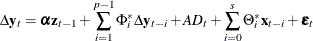
The VARX(p,s) model can be written as the error correction model
where
 ,
,  ,
,  , and
, and  are coefficient parameters;
  is a deterministic term such as a constant, a linear trend, or seasonal dummies.
The
 model is defined by one reduced-rank condition. If the cointegration rank is
  , then there exist
  matrices
  and
and  of rank r such that
  .
.
The
model is rewritten as the  model
model
where
 and
and 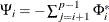 .
.
The
model is defined by two reduced-rank conditions. One is that , where and are matrices of full-rank r. The other is that  where
where  and
and  are
are  matrices with
  ;
;  and
and  are
are  matrices of full-rank
  such that
  and
and  .
.
The following options can be used in the JOHANSEN=( ) option. The options are specified within parentheses.
- IORDER=number
-
specifies the integrated order.
- IORDER=1
-
prints the cointegration rank test for an integrated order 1 and prints the long-run parameter,
, and the adjustment coefficient, . This is the default. If the IORDER=1 option is specified, then the AR order should be greater than or equal to 1. When the
P=0 option, the value of P is set to 1 for the Johansen test.
- IORDER=2
-
prints the cointegration rank test for integrated orders 1 and 2. If the IORDER=2 option is specified, then the AR order should be greater than or equal to 2. If the P=1 option with the IORDER=2 option, then the value of IORDER is set to 1; if the P=0 option with the IORDER=2 option, then the value of P is set to 2.
- NORMALIZE=variable
-
specifies the dependent (endogenous) variable name whose cointegration vectors are to be normalized. If the normalized variable is different from that specified in the ECM= option or the COINTEG statement, then the value specified in the COINTEG statement is used.
- TYPE=value
-
specifies the type of cointegration rank test to be printed. Valid values are as follows:
- MAX
-
prints the cointegration maximum eigenvalue test.
- TRACE
-
prints the cointegration trace test. This is the default.
If the NOINT option is not specified, the procedure prints two different cointegration rank tests in the presence of the unrestricted and restricted deterministic terms (constant or linear trend) models. If the IORDER=2 option is specified, the procedure automatically determines that the TYPE=TRACE option.
Some examples that illustrate the COINTTEST= option follow:
   model y1 y2 / p=2 cointtest=(johansen=(type=max normalize=y1));
   model y1 y2 / p=2 cointtest=(johansen=(iorder=2 normalize=y1));
- SIGLEVEL=value
-
sets the size, or the significance level, of common trends tests.The SIGLEVEL=value can be set to 0.1, 0.05, or 0.01. The default is SIGLEVEL=0.05.
   model y1 y2 / p=2 cointtest=(sw siglevel=0.1);
   model y1 y2 / p=2 cointtest=(sw siglevel=0.01);
-
SW
SW=(TYPE=value LAG=number) -
prints common trends tests for a multivariate time series based on the Stock-Watson method. This test is provided when the number of dependent (endogenous) variables is less than or equal to 6. See the section Common Trends for details.
The following options can be used in the SW=( ) option. The options are listed within parentheses.
- LAG=number
-
specifies the number of lags. The default is LAG=max(1,p) for the TYPE=FILTDIF or TYPE=FILTRES option, where p is the AR maximum order specified by the P= option; LAG=
 for the TYPE=KERNEL option, where is the number of nonmissing observations. If the specified LAG=number exceeds the default, then it is replaced by the default.
- TYPE=value
-
specifies the type of common trends test to be printed. Valid values are as follows:
- FILTDIF
-
prints the common trends test based on the filtering method applied to the differenced series. This is the default.
- FILTRES
-
prints the common trends test based on the filtering method applied to the residual series.
- KERNEL
-
prints the common trends test based on the kernel method.
   model y1 y2 / p=2 cointtest=(sw);
   model y1 y2 / p=2 cointtest=(sw=(type=kernel));
   model y1 y2 / p=2 cointtest=(sw=(type=kernel lag=3));
-
PRIOR
PRIOR=(prior-options) -
specifies the prior value of parameters for the BVARX(p, s) model. The BVARX model allows for a subset model specification. If the ECM= option is specified with the PRIOR option, the BVECMX(p, s) form is fitted. See the section Bayesian VAR and VARX Modeling for details.
The following options can be used with the PRIOR=(prior-options) option. The prior-options are listed within parentheses.
-
IVAR
IVAR=(variables) -
specifies an integrated BVAR(p) model. The variables should be specified in the MODEL statement as dependent variables. If you use the IVAR option without variables, then it sets the overall prior mean of the first lag of each variable equal to one in its own equation and sets all other coefficients to zero. If variables are specified, it sets the prior mean of the first lag of the specified variables equal to one in its own equation and sets all other coefficients to zero. When the series
 follows a bivariate BVAR(2) process, the IVAR or IVAR=(
  ) option is equivalent to specifying MEAN=(1 0 0 0 0 1 0 0).
If the PRIOR=(MEAN=) or ECM= option is specified, the IVAR= option is ignored.
- LAMBDA=value
-
specifies the prior standard deviation of the AR coefficient parameter matrices. It should be a positive number. The default is LAMBDA=1. As the value of the LAMBDA= option is increased, the BVAR(p) model becomes closer to a VAR(p) model.
- MEAN=(vector)
-
specifies the mean vector in the prior distribution for the AR coefficients. If the vector is not specified, the prior value is assumed to be a zero vector. See the section Bayesian VAR and VARX Modeling for details.
You can specify the mean vector by order of the equation. Let
 be the parameter sets to be estimated and
  be the AR parameter sets. The mean vector is specified by row-wise from
  ; that is, the MEAN=(
 ) option.
For the PRIOR=(mean) option in the BVAR(2),

where
 is an element of , l is a lag, i is associated with the first dependent variable, and j is associated with the second dependent variable.
model y1 y2 / p=2 prior=(mean=(2 0.1 1 0 0.5 3 0 -1));
The deterministic terms and exogenous variables are considered to shrink toward zero; you must omit prior means of exogenous variables and deterministic terms such as a constant, seasonal dummies, or trends.
For a Bayesian error correction model estimated when both the ECM= and PRIOR= options are used, a mean vector for only lagged AR coefficients,
, in terms of regressors  , for
, for  is used in the VECM(p) representation. The diffused prior variance of is used, since is replaced by
  estimated in a nonconstrained VECM(p) form.
where
 .
.
For example, in the case of a bivariate (
 ) BVECM(2) form, the option
![\[ \mr{MEAN} =( \phi ^*_{1,11} ~ \phi ^*_{1,12} ~ \phi ^*_{1,21} ~ \phi ^*_{1,22} ) \]](images/etsug_varmax0186.png)
where
 is the
  th element of the matrix
  .
.
- NREP=number
-
determines the number of repetitions that are used to compute the measure of forecast accuracy. See the equation in the section Forecasting of BVAR Modeling for details. The default is NREP=
 , where is the number of observations. If NREP is above , it is decreased to ; if NREP is below the value of the LEAD= option, it is increased to the value of the LEAD= option.
- THETA=value
-
specifies the prior standard deviation of the AR coefficient parameter matrices. The value is in the interval (0,1). The default is THETA=0.1. As the value of the THETA= option approaches 1, the specified BVAR(p) model approaches a VAR(p) model.
Some examples of the PRIOR= option follow:
   model y1 y2 / p=2 prior;
   model y1 y2 / p=2 prior=(theta=0.2 lambda=5);
   model y1 y2 = x1 / p=2 prior=(theta=0.2 lambda=5);
   model y1 y2 = x1 / p=2
      prior=(theta=0.2 lambda=5 mean=(2 0.1 1 0 0.5 3 0 -1));
See the section Bayesian VAR and VARX Modeling for details.
- ECM=(RANK=number NORMALIZE=variable ECTREND )
-
specifies a vector error correction model.
The following options can be used in the ECM=( ) option. The options are specified within parentheses.
- NORMALIZE=variable
-
specifies a single dependent variable name whose cointegrating vectors are normalized. If the variable name is different from that specified in the COINTEG statement, then the value specified in the COINTEG statement is used.
- RANK=number
-
specifies the cointegration rank. This option is required in the ECM= option. The value of the RANK= option should be greater than zero and less than or equal to the number of dependent (endogenous) variables, k. If the rank is different from that specified in the COINTEG statement, then the value specified in the COINTEG statement is used.
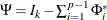
- ECTREND
-
specifies the restriction on the drift in the VECM(p) form.
-
There is no separate drift in the VECM(p) form, but a constant enters only through the error correction term.
![\[ \Delta \mb{y} _ t = \balpha (\bbeta ’, \beta _0)(\mb{y} _{t-1}’,1)’ + \sum _{i=1}^{p-1} \Phi ^*_ i \Delta \mb{y} _{t-i} + \bepsilon _ t \]](images/etsug_varmax0190.png)
An example of the ECTREND option follows:
model y1 y2 / p=2 ecm=(rank=1 ectrend);
-
There is a separate drift and no separate linear trend in the VECM(p) form, but a linear trend enters only through the error correction term.
![\[ \Delta \mb{y} _ t = \balpha (\bbeta ’, \beta _1)(\mb{y} _{t-1}’,t)’ + \sum _{i=1}^{p-1} \Phi ^*_ i \Delta \mb{y} _{t-i} + \bdelta _0 + \bepsilon _ t \]](images/etsug_varmax0191.png)
An example of the ECTREND option with the TREND= option follows:
model y1 y2 / p=2 ecm=(rank=1 ectrend) trend=linear;
If the NSEASON option is specified, then the NSEASON option is ignored; if the NOINT option is specified, then the ECTREND option is ignored.
Some examples of the ECM= option follow:
   model y1 y2 / p=2 ecm=(rank=1 normalized=y1);
   model y1 y2 / p=2 ecm=(rank=1 ectrend) trend=linear;
See the section Vector Error Correction Modeling for details.
-