The VARMAX Procedure
- Overview
-
Getting Started

-
Syntax
-
DetailsMissing ValuesVARMAX ModelDynamic Simultaneous Equations ModelingImpulse Response FunctionForecastingTentative Order SelectionVAR and VARX ModelingBayesian VAR and VARX ModelingVARMA and VARMAX ModelingModel Diagnostic ChecksCointegrationVector Error Correction ModelingI(2) ModelMultivariate GARCH ModelingOutput Data SetsOUT= Data SetOUTEST= Data SetOUTHT= Data SetOUTSTAT= Data SetPrinted OutputODS Table NamesODS GraphicsComputational Issues
-
Examples
- References
Stochastic volatility modeling is important in many areas, particularly in finance. To study the volatility of time series, GARCH models are widely used because they provide a good approach to conditional variance modeling.
Engle and Kroner (1995) propose a general multivariate GARCH model and call it a BEKK representation. Let ![]() be the sigma field generated by the past values of
be the sigma field generated by the past values of ![]() , and let
, and let ![]() be the conditional covariance matrix of the k-dimensional random vector
be the conditional covariance matrix of the k-dimensional random vector ![]() . Let
. Let ![]() be measurable with respect to
be measurable with respect to ![]() ; then the multivariate GARCH model can be written as
; then the multivariate GARCH model can be written as
where C, ![]() and
and ![]() are
are ![]() parameter matrices.
parameter matrices.
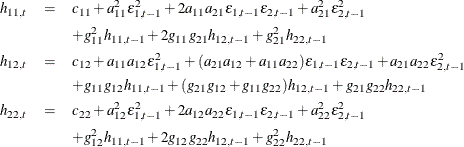
Consider the bivariate GARCH(1,1) model
![\begin{eqnarray*} H_ t & =& \left[ \begin{array}{cc} c_{11} & c_{12} \\ c_{12} & c_{22} \end{array} \right] +\left[ \begin{array}{cc} a_{11} & a_{12} \\ a_{21} & a_{22} \end{array} \right]’ \left[ \begin{array}{cc}\epsilon ^2_{1,t-1} & \epsilon _{1,t-1}\epsilon _{2,t-1} \\ \epsilon _{2,t-1}\epsilon _{1,t-1} & \epsilon ^2_{2,t-1} \end{array} \right] \left[ \begin{array}{cc} a_{11} & a_{12} \\ a_{21} & a_{22} \end{array} \right] \\ & & + \left[ \begin{array}{cc} g_{11} & g_{12} \\ g_{21} & g_{22} \end{array} \right]’ H_{t-1}\left[ \begin{array}{cc} g_{11} & g_{12} \\ g_{21} & g_{22} \end{array} \right] \end{eqnarray*}](images/etsug_varmax0929.png)
or, representing the univariate model,
For the BEKK representation of the bivariate GARCH(1,1) model, the SAS statements are
model y1 y2;
garch q=1 p=1 form=bekk;
The multistep forecast of the conditional covariance matrix, ![]() , is obtained recursively through the formula
, is obtained recursively through the formula
where ![]() for
for ![]() .
.
Bollerslev (1990) proposes a multivariate GARCH model with time-varying conditional variances and covariances but constant conditional correlations.
The conditional covariance matrix ![]() consists of
consists of
where ![]() is a
is a ![]() stochastic diagonal matrix with element
stochastic diagonal matrix with element ![]() and
and ![]() is a
is a ![]() time-invariant correlation matrix with the typical element
time-invariant correlation matrix with the typical element ![]() .
.
The element of ![]() is
is
Note that ![]() .
.
If you specify CORRCONSTANT=EXPECT, the element ![]() of the time-invariant correlation matrix
of the time-invariant correlation matrix ![]() is
is
where ![]() is the sample size.
is the sample size.
By default, or when you specify SUBFORM=GARCH, ![]() follows a univariate GARCH process,
follows a univariate GARCH process,
As shown in many empirical studies, positive and negative innovations have different impacts on future volatility. There is a long list of variations of univariate GARCH models that consider the asymmetricity. Four typical variations follow:
For more information about the asymmetric GARCH models, see Engle and Ng (1993). You can choose the type of GARCH model of interest by specifying the SUBFORM= option.
The EGARCH model was proposed by Nelson (1991). Nelson and Cao (1992) argue that the nonnegativity constraints in the GARCH model are too restrictive. The GARCH model, implicitly or explicitly, imposes the nonnegative constraints on the parameters, whereas these parameters have no restrictions in the EGARCH model. In the EGARCH model, the conditional variance is an asymmetric function of lagged disturbances,
In the QGARCH model, the lagged errors’ centers are shifted from zero to some constant values,
In the TGARCH model, each lagged squared error has an extra slope coefficient,
where the indicator function ![]() is one if
is one if ![]() and zero otherwise.
and zero otherwise.
The PGARCH model not only considers the asymmetric effect but also provides a way to model the long memory property in the volatility,
where ![]() and
and ![]() .
.
Note that the implemented TGARCH model is also well known as GJR-GARCH (Glosten, Jaganathan, and Runkle, 1993), which is similar to the threshold GARCH model proposed by Zakoian (1994) but not exactly the same. In Zakoian’s model, the conditional standard deviation is a linear function of the past values
of the white noise. Zakoian’s model can be regarded as a special case of the PGARCH model when ![]() .
.
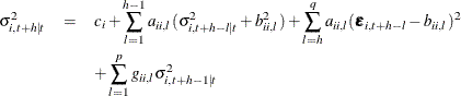
The following formulas are recursively implemented to obtain the multistep forecast of conditional error variance ![]() and
and ![]() :
:
-
for the GARCH(p, q) model:

-
for the EGARCH(p, q) model:

-
for the QGARCH(p, q) model:
-
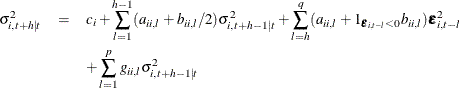
for the TGARCH(p, q) model:
-
for the PGARCH(p, q) model:
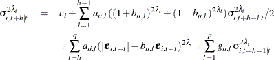
In the preceding equations, ![]() for
for ![]() . Then, the multistep forecast of conditional covariance matrix
. Then, the multistep forecast of conditional covariance matrix ![]() , is calculated by
, is calculated by
where ![]() is the diagonal matrix with element
is the diagonal matrix with element ![]() .
.
Engle (2002) proposes a parsimonious parametric multivariate GARCH model that has time-varying conditional covariances and correlations.
The conditional covariance matrix ![]() consists of
consists of
where ![]() is a
is a ![]() stochastic diagonal matrix with the element
stochastic diagonal matrix with the element ![]() and
and ![]() is a
is a ![]() time-varying matrix with the typical element
time-varying matrix with the typical element ![]() .
.
The element of ![]() is
is
Note that ![]() .
.
As in the CCC GARCH model, you can choose the type of GARCH model of interest by specifying the SUBFORM= option.
In the GARCH model,
In the EGARCH model, the conditional variance is an asymmetric function of lagged disturbances,
In the QGARCH model, the lagged errors’ centers are shifted from zero to some constant values,
In the TGARCH model, each lagged squared error has an extra slope coefficient,
where the indicator function ![]() is one if
is one if ![]() and zero otherwise.
and zero otherwise.
The PGARCH model not only considers the asymmetric effect but also provides another way to model the long memory property in the volatility,
where ![]() and
and ![]() .
.
The conditional correlation estimator ![]() is
is
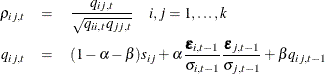
where ![]() is the element of
is the element of ![]() , the unconditional correlation matrix.
, the unconditional correlation matrix.
If you specify CORRCONSTANT=EXPECT, the element ![]() of the unconditional correlation matrix
of the unconditional correlation matrix ![]() is
is
where ![]() is the sample size.
is the sample size.
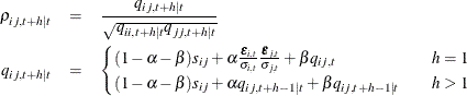
As shown in the CCC GARCH models, the following formulas are recursively implemented to obtain the multistep forecast of conditional
error variance ![]() and
and ![]() :
:
-
for the GARCH(p, q) model:
-
for the EGARCH(p, q) model:
-
for the QGARCH(p, q) model:
-
for the TGARCH(p, q) model:
-
for the PGARCH(p, q) model:
In the preceding equations, ![]() for
for ![]() . Then, the multistep forecast of conditional covariance matrix
. Then, the multistep forecast of conditional covariance matrix ![]() , is calculated by
, is calculated by
where ![]() is the diagonal matrix with element
is the diagonal matrix with element ![]() , and
, and ![]() is the matrix with element
is the matrix with element ![]() ,
,
The log-likelihood function of the multivariate GARCH model is written without a constant term as
The log-likelihood function is maximized by an iterative numerical method such as quasi-Newton optimization. The starting
values for the regression parameters are obtained from the least squares estimates. The covariance of ![]() is used as the starting values for the GARCH constant parameters, and the starting value for the other GARCH parameters is
either
is used as the starting values for the GARCH constant parameters, and the starting value for the other GARCH parameters is
either ![]() or
or ![]() , depending on the GARCH model’s representation.
, depending on the GARCH model’s representation.
In multivariate GARCH models, the optimal (minimum MSE) l-step-ahead forecast of endogenous variables ![]() uses the same formula as shown in the section Forecasting. However, the exogenous (independent) variables, if present, are always assumed to be nonstochastic (deterministic); that
is, to predict the endogenous variables, you must specify the future values of the exogenous variables. The prediction error
of the optimal l-step-ahead forecast is
uses the same formula as shown in the section Forecasting. However, the exogenous (independent) variables, if present, are always assumed to be nonstochastic (deterministic); that
is, to predict the endogenous variables, you must specify the future values of the exogenous variables. The prediction error
of the optimal l-step-ahead forecast is ![]() , with zero mean and covariance matrix,
, with zero mean and covariance matrix,
where ![]() is the h-step-ahead forecast of the conditional covariance matrix. As emphasized by the subscript t,
is the h-step-ahead forecast of the conditional covariance matrix. As emphasized by the subscript t, ![]() is time-dependent. In the OUT= data set, the forecast standard errors and prediction intervals are constructed according
to
is time-dependent. In the OUT= data set, the forecast standard errors and prediction intervals are constructed according
to ![]() . If you specify the COVPE option, the prediction error covariances that are output in the CovPredictError and CovPredictErrorbyVar
ODS tables are based on the time-independent formula
. If you specify the COVPE option, the prediction error covariances that are output in the CovPredictError and CovPredictErrorbyVar
ODS tables are based on the time-independent formula
where ![]() is the unconditional covariance matrix of innovations. The decomposition of the prediction error covariances is also based
on
is the unconditional covariance matrix of innovations. The decomposition of the prediction error covariances is also based
on ![]() .
.
Define the multivariate GARCH process as
where ![]() ,
, ![]() , and
, and ![]() . This representation is equivalent to a GARCH(
. This representation is equivalent to a GARCH(![]() ) model by the following algebra:
) model by the following algebra:
![\begin{eqnarray*} \mb{h}_ t & =& \mb{c} + A(B)\bm {\eta }_ t + \sum _{i=2}^\infty G(B)^{i-1}[\mb{c} +A(B)\bm {\eta }_ t] \\ & =& \mb{c} + A(B)\bm {\eta }_ t + G(B)\sum _{i=1}^\infty G(B)^{i-1}[tmb{c} +A(B)\bm {\eta }_ t] \\ & =& \mb{c} + A(B)\bm {\eta }_ t + G(B) \mb{h}_ t \end{eqnarray*}](images/etsug_varmax0989.png)
Defining ![]() and
and ![]() gives a BEKK representation.
gives a BEKK representation.
The necessary and sufficient conditions for covariance stationarity of the multivariate GARCH process are that all the eigenvalues
of ![]() are less than 1 in modulus.
are less than 1 in modulus.
The following DATA step simulates a bivariate vector time series to provide test data for the multivariate GARCH model:
data garch;
   retain seed 16587;
   esq1 = 0; esq2 = 0;
   ly1 = 0;  ly2 = 0;
   do i = 1 to 1000;
      ht = 6.25 + 0.5*esq1;
      call rannor(seed,ehat);
      e1 = sqrt(ht)*ehat;
      ht = 1.25 + 0.7*esq2;
      call rannor(seed,ehat);
      e2 = sqrt(ht)*ehat;
      y1 = 2 + 1.2*ly1 - 0.5*ly2 + e1;
      y2 = 4 + 0.6*ly1 + 0.3*ly2 + e2;
      if i>500 then output;
      esq1 = e1*e1; esq2 = e2*e2;
      ly1 = y1;  ly2 = y2;
   end;
   keep y1 y2;
run;
The following statements fit a VAR(1)–ARCH(1) model to the data. For a VAR-ARCH model, you specify the order of the autoregressive model with the P=1 option in the MODEL statement and the Q=1 option in the GARCH statement. In order to produce the initial and final values of parameters, the TECH=QN option is specified in the NLOPTIONS statement.
proc varmax data=garch;
   model y1 y2 / p=1
         print=(roots estimates diagnose);
   garch q=1;
   nloptions tech=qn;
run;
Figure 35.61 through Figure 35.65 show the details of this example. Figure 35.61 shows the initial values of parameters.
Figure 35.61: Start Parameter Estimates for the VAR(1)–ARCH(1) Model
| Optimization Start | |||
|---|---|---|---|
| Parameter Estimates | |||
| N | Parameter | Estimate | Gradient Objective Function |
| 1 | CONST1 | 2.249575 | 0.000082533 |
| 2 | CONST2 | 3.902673 | 0.000401 |
| 3 | AR1_1_1 | 1.231775 | 0.000105 |
| 4 | AR1_2_1 | 0.576890 | -0.004811 |
| 5 | AR1_1_2 | -0.528405 | 0.000617 |
| 6 | AR1_2_2 | 0.343714 | 0.001811 |
| 7 | GCHC1_1 | 9.929763 | 0.151293 |
| 8 | GCHC1_2 | 0.193163 | -0.014305 |
| 9 | GCHC2_2 | 4.063245 | 0.370333 |
| 10 | ACH1_1_1 | 0.001000 | -0.667182 |
| 11 | ACH1_2_1 | 0 | -0.068905 |
| 12 | ACH1_1_2 | 0 | -0.734486 |
| 13 | ACH1_2_2 | 0.001000 | -3.127035 |
Figure 35.62 shows the final parameter estimates.
Figure 35.62: Results of Parameter Estimates for the VAR(1)–ARCH(1) Model
| Optimization Results | |||
|---|---|---|---|
| Parameter Estimates | |||
| N | Parameter | Estimate | Gradient Objective Function |
| 1 | CONST1 | 2.156865 | 0.000246 |
| 2 | CONST2 | 4.048879 | 0.000105 |
| 3 | AR1_1_1 | 1.224620 | -0.001957 |
| 4 | AR1_2_1 | 0.609651 | 0.000173 |
| 5 | AR1_1_2 | -0.534248 | -0.000468 |
| 6 | AR1_2_2 | 0.302599 | -0.000375 |
| 7 | GCHC1_1 | 8.238625 | -0.000056090 |
| 8 | GCHC1_2 | -0.231183 | -0.000021724 |
| 9 | GCHC2_2 | 1.565459 | 0.000110 |
| 10 | ACH1_1_1 | 0.374255 | -0.000419 |
| 11 | ACH1_2_1 | 0.035883 | -0.000606 |
| 12 | ACH1_1_2 | 0.057461 | 0.001636 |
| 13 | ACH1_2_2 | 0.717897 | -0.000149 |
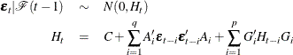
Figure 35.63 shows the conditional variance by using the BEKK representation of the ARCH(1) model. The ARCH parameters are estimated as follows by the vectorized parameter matrices:
![\begin{eqnarray*} \bepsilon _ t|\mathcal{F}(t-1) & \sim & N(0,H_ t) \\ H_ t & = & \left[ \begin{matrix} 8.23863 & -0.23118 \\ -0.23118 & 1.56546 \\ \end{matrix} \right] \\ & + & \left[ \begin{matrix} 0.37426 & 0.05746 \\ 0.03588 & 0.71790 \\ \end{matrix} \right]’ \bepsilon _{t-1}\bepsilon _{t-1}’ \left[ \begin{matrix} 0.37426 & 0.05746 \\ 0.03588 & 0.71790 \\ \end{matrix} \right] \end{eqnarray*}](images/etsug_varmax0993.png)
Figure 35.63: ARCH(1) Parameter Estimates for the VAR(1)–ARCH(1) Model
| Type of Model | VAR(1)-ARCH(1) |
|---|---|
| Estimation Method | Maximum Likelihood Estimation |
| Representation Type | BEKK |
| GARCH Model Parameter Estimates | ||||
|---|---|---|---|---|
| Parameter | Estimate | Standard Error |
t Value | Pr > |t| |
| GCHC1_1 | 8.23863 | 0.72663 | 11.34 | 0.0001 |
| GCHC1_2 | -0.23118 | 0.21434 | -1.08 | 0.2813 |
| GCHC2_2 | 1.56546 | 0.19407 | 8.07 | 0.0001 |
| ACH1_1_1 | 0.37426 | 0.07502 | 4.99 | 0.0001 |
| ACH1_2_1 | 0.03588 | 0.06974 | 0.51 | 0.6071 |
| ACH1_1_2 | 0.05746 | 0.02597 | 2.21 | 0.0274 |
| ACH1_2_2 | 0.71790 | 0.06895 | 10.41 | 0.0001 |
Figure 35.64 shows the AR parameter estimates and their significance.
The fitted VAR(1) model with the previous conditional covariance ARCH model is written as follows:
Figure 35.64: VAR(1) Parameter Estimates for the VAR(1)–ARCH(1) Model
| Model Parameter Estimates | ||||||
|---|---|---|---|---|---|---|
| Equation | Parameter | Estimate | Standard Error |
t Value | Pr > |t| | Variable |
| y1 | CONST1 | 2.15687 | 0.21717 | 9.93 | 0.0001 | 1 |
| AR1_1_1 | 1.22462 | 0.02542 | 48.17 | 0.0001 | y1(t-1) | |
| AR1_1_2 | -0.53425 | 0.02807 | -19.03 | 0.0001 | y2(t-1) | |
| y2 | CONST2 | 4.04888 | 0.10663 | 37.97 | 0.0001 | 1 |
| AR1_2_1 | 0.60965 | 0.01216 | 50.13 | 0.0001 | y1(t-1) | |
| AR1_2_2 | 0.30260 | 0.01491 | 20.30 | 0.0001 | y2(t-1) | |
Figure 35.65 shows the roots of the AR and ARCH characteristic polynomials. The eigenvalues have a modulus less than one.
Figure 35.65: Roots for the VAR(1)–ARCH(1) Model
| Roots of AR Characteristic Polynomial | |||||
|---|---|---|---|---|---|
| Index | Real | Imaginary | Modulus | Radian | Degree |
| 1 | 0.76361 | 0.33641 | 0.8344 | 0.4150 | 23.7762 |
| 2 | 0.76361 | -0.33641 | 0.8344 | -0.4150 | -23.7762 |
| Roots of GARCH Characteristic Polynomial | |||||
|---|---|---|---|---|---|
| Index | Real | Imaginary | Modulus | Radian | Degree |
| 1 | 0.52388 | 0.00000 | 0.5239 | 0.0000 | 0.0000 |
| 2 | 0.26661 | 0.00000 | 0.2666 | 0.0000 | 0.0000 |
| 3 | 0.26661 | 0.00000 | 0.2666 | 0.0000 | 0.0000 |
| 4 | 0.13569 | 0.00000 | 0.1357 | 0.0000 | 0.0000 |