The BOXPLOT Procedure

The previous example illustrates how you can create box plots from raw data. However, in some applications the data are provided as summary statistics. This example illustrates how you can use the BOXPLOT procedure with data of this type.
The following statements create the data set Oilsum, which provides the data from the preceding example in summarized form:
data Oilsum;
   input Day KWattsL KWatts1 KWattsX KWattsM
             KWatts3 KWattsH KWattsS KWattsN;
   informat Day date7. ;
   format Day date5. ;
   label Day    ='Date of Measurement'
         KWattsL='Minimum Power Output'
         KWatts1='25th Percentile'
         KWattsX='Average Power Output'
         KWattsM='Median Power Output'
         KWatts3='75th Percentile'
         KWattsH='Maximum Power Output'
         KWattsS='Standard Deviation of Power Output'
         KWattsN='Group Sample Size';
   datalines;
05JUL94 3180 3340.0 3487.40 3490.0 3610.0 4050 220.3 20
06JUL94 3179 3333.5 3471.65 3419.5 3605.0 3849 210.4 20
07JUL94 3304 3376.0 3488.30 3456.5 3604.5 3781 147.0 20
08JUL94 3045 3390.5 3434.20 3447.0 3550.0 3629 157.6 20
11JUL94 2968 3321.0 3475.80 3487.0 3611.5 3916 258.9 20
12JUL94 3047 3425.5 3518.10 3576.0 3615.0 3881 211.6 20
13JUL94 3002 3368.5 3492.65 3495.5 3621.5 3787 193.8 20
14JUL94 3196 3346.0 3496.40 3473.5 3592.5 3994 212.0 20
15JUL94 3115 3188.5 3398.50 3426.0 3568.5 3731 199.2 20
18JUL94 3263 3340.0 3456.05 3444.0 3505.5 4040 173.5 20
;
Oilsum contains exactly one observation for each group. Note that, as in the previous example, the groups are indexed by the variable
Day. A listing of Oilsum is shown in Figure 26.2.
Figure 26.2: The Summary Data Set Oilsum
| Box Plot for Power Output |
| Day | KWattsL | KWatts1 | KWattsX | KWattsM | KWatts3 | KWattsH | KWattsS | KWattsN |
|---|---|---|---|---|---|---|---|---|
| 05JUL | 3180 | 3340.0 | 3487.40 | 3490.0 | 3610.0 | 4050 | 220.3 | 20 |
| 06JUL | 3179 | 3333.5 | 3471.65 | 3419.5 | 3605.0 | 3849 | 210.4 | 20 |
| 07JUL | 3304 | 3376.0 | 3488.30 | 3456.5 | 3604.5 | 3781 | 147.0 | 20 |
| 08JUL | 3045 | 3390.5 | 3434.20 | 3447.0 | 3550.0 | 3629 | 157.6 | 20 |
| 11JUL | 2968 | 3321.0 | 3475.80 | 3487.0 | 3611.5 | 3916 | 258.9 | 20 |
| 12JUL | 3047 | 3425.5 | 3518.10 | 3576.0 | 3615.0 | 3881 | 211.6 | 20 |
| 13JUL | 3002 | 3368.5 | 3492.65 | 3495.5 | 3621.5 | 3787 | 193.8 | 20 |
| 14JUL | 3196 | 3346.0 | 3496.40 | 3473.5 | 3592.5 | 3994 | 212.0 | 20 |
| 15JUL | 3115 | 3188.5 | 3398.50 | 3426.0 | 3568.5 | 3731 | 199.2 | 20 |
| 18JUL | 3263 | 3340.0 | 3456.05 | 3444.0 | 3505.5 | 4040 | 173.5 | 20 |
There are eight summary variables in Oilsum:
-
KWattsLcontains the group minima (low values). -
KWatts1contains the 25th percentile (first quartile) for each group. -
KWattsXcontains the group means. -
KWattsMcontains the group medians. -
KWatts3contains the 75th percentile (third quartile) for each group. -
KWattsHcontains the group maxima (high values). -
KWattsScontains the group standard deviations. -
KWattsNcontains the group sizes.
You can use this data set as input to the BOXPLOT procedure by specifying it with the HISTORY= option in the PROC BOXPLOT statement. Detailed requirements for HISTORY= data sets are presented in the section HISTORY= Data Set.
The following statements produce a box plot of the summary data from the Oilsum data set:
options nogstyle;
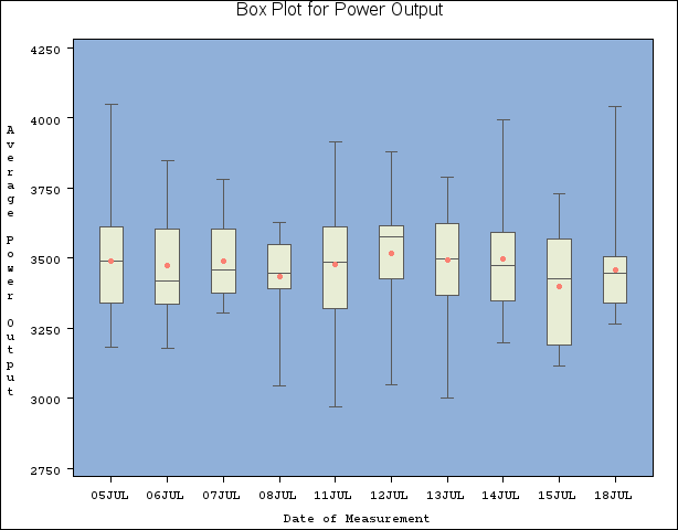
title 'Box Plot for Power Output';
symbol value=dot color=salmon;
proc boxplot history=Oilsum;
plot KWatts*Day / cframe = vligb
cboxes = dagr
cboxfill = ywh;
run;
options gstyle;
goptions reset=symbol;
The NOGSTYLE system option causes PROC BOXPLOT to ignore ODS styles when producing the box plot. Instead, the SYMBOL statement and options specified after the slash (/) in the PLOT statement control its appearance. The GSTYLE system option restores the use of ODS styles for subsequent high-resolution graphics output. For more information about SYMBOL statements, see SAS/GRAPH: Reference. The resulting box plot is shown in Figure 26.3.