The BCHOICE Procedure

Discrete Choice Models
Discrete choice models are used in marketing research to model decision makers’ choices among alternative products and services. The decision makers might be people, households, companies and so on, and the alternatives might be products, services, actions, or any other options or items about which choices must be made (Train 2009). The collection of alternatives that are available to the decision makers is called a choice set.
Discrete choice models are derived under the assumption of utility-maximizing behavior by the decision maker. When individuals are asked to make one choice among a set of alternatives, they usually determine the level of utility that each alternative offers. The utility that individual i obtains from alternative j among J alternatives is denoted as
![\[ u_{ij} = v_{ij} + \epsilon _{ij}, ~ ~ ~ ~ i=1, \ldots , N, ~ ~ \mbox{and}~ ~ j=1, \ldots , J \]](images/statug_bchoice0071.png)
where the subscript i is an index for the individuals, the subscript j is an index for the alternatives in a choice set,  is a nonstochastic utility function that relates those observed factors to the utility, and
  is the error component that captures the unobserved characteristics of the utility. In discrete choice models, the observed
part of the utility function is assumed to be linear in the parameters,
is the error component that captures the unobserved characteristics of the utility. In discrete choice models, the observed
part of the utility function is assumed to be linear in the parameters,
![\[ v_{ij}=\mb{x}_{ij}’\bbeta \]](images/statug_bchoice0004.png)
where  is a p-dimensional design vector of observed attribute levels that relate to alternative j and
  is the corresponding vector of fixed regression coefficients that indicate the utilities or part-worths of the attribute
levels.
is the corresponding vector of fixed regression coefficients that indicate the utilities or part-worths of the attribute
levels.
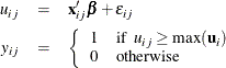
Decision makers choose the alternative that gives them the greatest utility. Let  be the multinomial response vector for the ith individual. The value
  takes 1 if the jth component of
 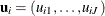 is the largest, and 0 otherwise:
The probability that the individual i chooses alternative j is
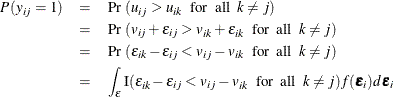
where I(.) is the indicator function and  denotes the joint density of the error vector
 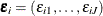 . Different specifications about the density result in different types of choice models, as detailed in the next section.
Logit and nested logit models have a closed form for this integral, whereas a probit model does not.
. Different specifications about the density result in different types of choice models, as detailed in the next section.
Logit and nested logit models have a closed form for this integral, whereas a probit model does not.