The MCMC Procedure

Example 61.6 Nonlinear Poisson Regression Models

This example illustrates how to fit a nonlinear Poisson regression with PROC MCMC. In addition, it shows how you can improve the mixing of the Markov chain by selecting a different proposal distribution or by sampling on the transformed scale of a parameter. This example shows how to analyze count data for calls to a technical support help line in the weeks immediately following a product release. This information could be used to decide upon the allocation of technical support resources for new products. You can model the number of daily calls as a Poisson random variable, with the average number of calls modeled as a nonlinear function of the number of weeks that have elapsed since the product’s release. The data are input into a SAS data set as follows:

title 'Nonlinear Poisson Regression';
data calls;
   input weeks calls @@;
   datalines;
1   0   1   2   2   2   2   1   3   1   3   3
4   5   4   8   5   5   5   9   6  17   6   9
7  24   7  16   8  23   8  27
;

During the first several weeks after a new product is released, the number of questions that technical support receives concerning the product increases in a sigmoidal fashion. The expression for the mean value in the classic Poisson regression involves the log link. There is some theoretical justification for this link, but with MCMC methodologies, you are not constrained to exploring only models that are computationally convenient. The number of calls to technical support tapers off after the initial release, so in this example you can use a logistic-type function to model the mean number of calls received weekly for the time period immediately following the initial release. The mean function $\lambda (t)$ is modeled as follows:

$\lambda _ i = \frac{\gamma }{1 + \exp \left[-(\alpha + \beta t_ i) \right]}$

The likelihood for every observation $\Variable{calls}_ i$ is

$\mbox{calls}_ i \sim \mbox{Poisson }(\lambda _ i)$

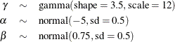
Past experience with technical support data for similar products suggests the following prior distributions:

$\begin{eqnarray*} \gamma & \sim & \mbox{gamma}(\mbox{shape} = 3.5, \mbox{scale} = 12) \\ \alpha & \sim & \mbox{normal}(-5, \mbox{sd} = 0.5) \\ \beta & \sim & \mbox{normal}(0.75, \mbox{sd} = 0.5) \end{eqnarray*}$

The following PROC MCMC statements fit this model:

ods graphics on;
proc mcmc data=calls outpost=callout seed=53197 ntu=1000 nmc=20000
       propcov=quanew stats=none diag=ess;
   ods select TADpanel ess;
   parms alpha -4 beta 1 gamma 2;
   prior gamma ~ gamma(3.5, scale=12);
   prior alpha ~ normal(-5, sd=0.25);
   prior beta  ~ normal(0.75, sd=0.5);
   lambda = gamma*logistic(alpha+beta*weeks);
   model calls ~ poisson(lambda);
run;

The one PARMS statement defines a block of all parameters and sets their initial values individually. The PRIOR statements specify the informative prior distributions for the three parameters. The assignment statement defines $\lambda$ , the mean number of calls. Instead of using the SAS function LOGISTIC, you can use the following statement to calculate $\lambda$ and get the same result:

lambda = gamma / (1 + exp(-(alpha+beta*weeks)));

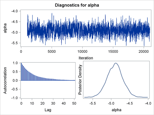
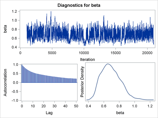
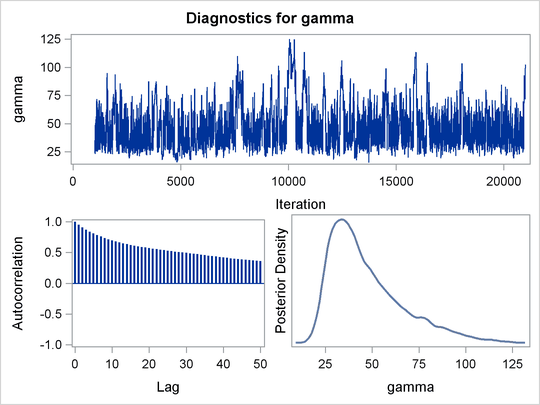
Mixing is not particularly good with this run of PROC MCMC. The ODS SELECT statement displays the diagnostic graphs and effective sample sizes (ESS) calculation while excluding all other output. The graphical output is shown in Output 61.6.1, and the ESS of each parameters are all relatively low (Output 61.6.2).

Output 61.6.1: Plots for Parameters

Output 61.6.2: Effective Sample Sizes

Nonlinear Poisson Regression

The MCMC Procedure

Effective Sample Sizes
Parameter	ESS	Autocorrelation Time	Efficiency
alpha	897.4	22.2870	0.0449
beta	231.6	86.3540	0.0116
gamma	162.9	122.8	0.0081

Often a simple scatter plot of the posterior samples can reveal a potential cause of the bad mixing. You can use PROC SGSCATTER to generate pairwise scatter plots of the three model parameters. The following statements generate Output 61.6.3:

proc sgscatter data=callout;
   matrix alpha beta gamma;
run;

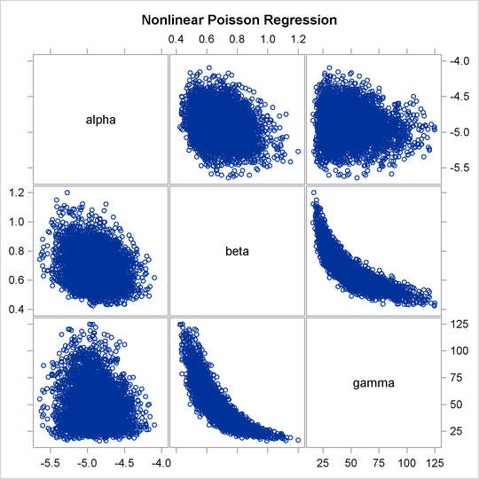
Output 61.6.3: Pairwise Scatter Plots of the Parameters

The nonlinearity in parameters beta and gamma stands out immediately. This explains why a random walk Metropolis with normal proposal has a difficult time exploring the joint distribution efficiently—the algorithm works best when the target distribution is unimodal and symmetric (normal-like). When there is nonlinearity in the parameters, it is impossible to find a single proposal scale parameter that optimally adapts to different regions of the joint parameter space. 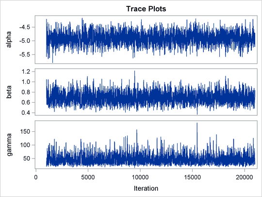As a result, the Markov chain can be inefficient in traversing some parts of the distribution. This is evident in examining the trace plot of the gamma parameter. You see that the Markov chain sometimes gets stuck in the far-right tail and does not travel back to the high-density area quickly. This effect can be seen around the simulations 8,000 and 18,000 in Output 61.6.1.

Reparameterization can often improve the mixing of the Markov chain. Note that the parameter gamma has a positive support and that the posterior distribution is right-skewed. This suggests that the chain might mix more rapidly if you sample on the logarithm of the parameter gamma.

Let $\delta = \log (\gamma )$ , and reparameterize the mean function as follows:

$\lambda _ i = \frac{\exp (\delta )}{1 + \exp \left[-(\alpha + \beta t_ i) \right]}$

To obtain the same inference, you use an induced prior on delta based on the gamma prior on the gamma parameter. This involves a transformation of variables, and you can obtain the following equivalency, where $|\exp (\delta )|$ is the Jacobian:

$\begin{eqnarray*} & & \pi (\gamma ) = \mbox{gamma}(\gamma ; a, \mbox{scale}=b) = \frac{1}{b^ a\Gamma (a)} \gamma ^{a-1} \exp \left( -\gamma /b \right) \\ & \Leftrightarrow & \pi (\delta ) = \mbox{gamma}(\gamma = \exp (\delta ); a, \mbox{scale}=b) \cdot \left| \exp (\delta ) \right| \end{eqnarray*}$

The distribution on $\delta$ simplifies to the following:

$\pi (\delta ) = \frac{1}{b^{a}\Gamma (a)} \exp \left(a \delta \right) \exp \left( - \exp \left(\delta \right) /b \right)$

PROC MCMC supports such a distribution on the logarithm transformation of a gamma random variable. It is called the ExpGamma distribution.

In the original model, you specify a prior on gamma:

prior gamma ~ gamma(3.5, scale=12);

You can obtain the same inference by specifying an ExpGamma prior on delta and take an exponential transformation to get back to gamma:

prior delta ~ egamma(3.5, scale=12);
gamma = exp(delta);

The following statements produce Output 61.6.6 and Output 61.6.4:

proc mcmc data=calls outpost=tcallout seed=53197 ntu=1000 nmc=20000
       propcov=quanew diag=ess plots=(trace) monitor=(alpha beta gamma);
   ods select PostSumInt ESS TRACEpanel;
   parms alpha -4 beta 1 delta 2;
   prior alpha ~ normal(-5, sd=0.25);
   prior beta  ~ normal(0.75, sd=0.5);
   prior delta ~ egamma(3.5, scale=12);
   gamma = exp(delta);
   lambda = gamma*logistic(alpha+beta*weeks);
   model calls ~ poisson(lambda);
run;

The PARMS statement declares delta, instead of gamma, as a model parameter. The prior distribution of delta is egamma, as opposed to the gamma distribution. The GAMMA assignment statement transforms delta to gamma. The LAMBDA assignment statement calculates the mean for the Poisson by using the gamma parameter. The MODEL statement specifies a Poisson likelihood for the calls response.

The trace plots in Output 61.6.4 show better mixing of the parameters, and the effective sample sizes in Output 61.6.5 show substantial improvements over the original formulation of the model. The improvements are especially obvious in beta and gamma, where the increase is fivefold to tenfold.

Output 61.6.4: Plots for Parameters, Sampling on the Log Scale of Gamma

Output 61.6.5: Effective Sample Sizes, Sampling on the Log Scale of Gamma

Nonlinear Poisson Regression

The MCMC Procedure

Effective Sample Sizes
Parameter	ESS	Autocorrelation Time	Efficiency
alpha	1338.4	14.9430	0.0669
beta	1254.9	15.9379	0.0627
gamma	1073.4	18.6320	0.0537

Output 61.6.6 shows the posterior summary and interval statistics of the nonlinear Poisson regression.

Output 61.6.6: MCMC Results, Sampling on the Log Scale of Gamma

Nonlinear Poisson Regression

The MCMC Procedure

Posterior Summaries and Intervals
Parameter	N	Mean	Standard Deviation	95% HPD Interval
alpha	20000	-4.9040	0.2234	-5.3217	-4.4544
beta	20000	0.6899	0.1154	0.4841	0.9169
gamma	20000	46.7199	19.4977	19.6588	86.2425

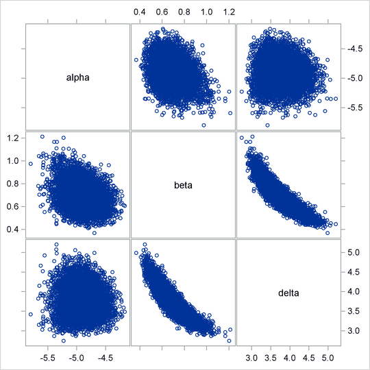
Note that the delta parameter has a more symmetric density than the skewed gamma parameter. A pairwise scatter plot (Output 61.6.7) shows a more linear relationship between beta and delta. The Metropolis algorithm always works better if the target distribution is approximately normal.

proc sgscatter data=tcallout;
   matrix alpha beta delta;
run;

Output 61.6.7: Pairwise Scatter Plots of the Transformed Parameters

If you are still unsatisfied with the slight nonlinearity in the parameters beta and delta, you can try another transformation on beta. Normally you would not want to do a logarithm transformation on a parameter that has support on the real axis, because you would risk taking the logarithm of negative values. However, because all the beta samples are positive and the marginal posterior distribution is away from 0, you can try a such a transformation.

Let $\kappa = \log (\beta )$ . The prior distribution on $\kappa$ is the following:

$\pi (\kappa ) = \mbox{normal}(\beta = \exp (\kappa ); \mu , \sigma ^2) \cdot \left| \exp (\kappa ) \right|$

You can specify the prior distribution in PROC MCMC by using a GENERAL function:

parms kappa;
lprior = logpdf("normal", exp(kappa), 0.75, 0.5) + kappa;
prior kappa ~ general(lp);
beta = exp(kappa);

The PARMS statement declares the transformed parameter kappa, which will be sampled. The LPRIOR assignment statement defines the logarithm of the prior distribution on kappa. The LOGPDF function is used here to simplify the specification of the distribution. The PRIOR statement specifies the nonstandard distribution as the prior on kappa. Finally, the BETA assignment statement transforms kappa back to the beta parameter.

Applying logarithm transformations on both beta and gamma yields the best mixing. (The results are not shown here, but you can find the code in the file mcmcex6.sas in the SAS Sample Library.) The transformed parameters kappa and delta have much clearer linear correlation. However, the improvement over the case where gamma alone is transformed is only marginally significant (50% increase in ESS).

This example illustrates that PROC MCMC can fit Bayesian nonlinear models just as easily as Bayesian linear models. More importantly, transformations can sometimes improve the efficiency of the Markov chain, and that is something to always keep in mind. Also see Using a Transformation to Improve Mixing for another example of how transformations can improve mixing of the Markov chains.