The MCMC Procedure

Usage of Multivariate Distributions

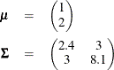
The following simple example illustrates the usage of the multivariate distributions in PROC MCMC. Suppose you are interested in estimating the mean and covariance of multivariate data using this multivariate normal model:

$\begin{pmatrix} \mbox{x}_1 \\ \mbox{x}_2 \end{pmatrix} \sim \mbox{MVN}\left(\bm {\mu } = \begin{pmatrix} \mu _1 \\ \mu _2 \end{pmatrix}, \bm {\Sigma } = \begin{pmatrix} \sigma _{11} & \sigma _{12} \\ \sigma _{21} & \sigma _{22} \end{pmatrix} \right)$

where

$\begin{eqnarray*} \bm {\mu } & =& \begin{pmatrix} 1 \\ 2 \end{pmatrix}\\ \bm {\Sigma } & =& \begin{pmatrix} 2.4 & 3 \\ 3 & 8.1 \end{pmatrix}\end{eqnarray*}$

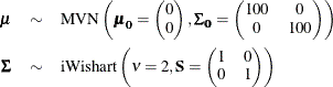
You can use the following independent prior on $\bm {\mu }$ and $\bm {\Sigma }$ :

$\begin{eqnarray*} \bm {\mu } & \sim & \mbox{MVN} \left( \bm {\mu _0} = \begin{pmatrix} 0 \\ 0 \end{pmatrix} , \bm {\Sigma _0} = \begin{pmatrix} 100 & 0 \\ 0 & 100 \end{pmatrix} \right) \\ \bm {\Sigma } & \sim & \mbox{iWishart} \left( \nu =2, \mb{S} = \left( \begin{matrix} 1 & 0 \\ 0 & 1 \end{matrix} \right) \right) \end{eqnarray*}$

The following IML procedure statements simulate 100 random multivariate normal samples:

title 'An Example that Uses Multivariate Distributions';
proc iml;
   N = 100;
   Mean = {1 2};
   Cov =  {2.4 3, 3 8.1};
   call randseed(1);
   x = RANDNORMAL( N, Mean, Cov );

   SampleMean = x[:,];
   n = nrow(x);
   y = x - repeat( SampleMean, n );
   SampleCov = y`*y / (n-1);
   print SampleMean Mean, SampleCov Cov;

   cname = {"x1", "x2"};
   create inputdata from x [colname = cname];
   append from x;
   close inputdata;
quit;

Figure 61.13 prints the sample mean and covariance of the simulated data, in addition to the true mean and covariance matrix.

Figure 61.13: Simulated Multivariate Normal Data

An Example that Uses Multivariate Distributions

SampleMean		Mean
0.9987751	2.115693	1	2

SampleCov		Cov
2.8252975	3.7190704	2.4	3
3.7190704	9.2916805	3	8.1

The following PROC MCMC statements estimate the posterior mean and covariance of the multivariate normal data:

proc mcmc data=inputdata seed=17 nmc=3000 diag=none;
   ods select PostSumInt;
   array data[2] x1 x2;
   array mu[2];
   array Sigma[2,2];
   array mu0[2] (0 0);
   array Sigma0[2,2] (100 0 0 100);
   array S[2,2] (1 0 0 1);
   parm mu Sigma;
   prior mu ~ mvn(mu0, Sigma0);
   prior Sigma ~ iwish(2, S);
   model data ~ mvn(mu, Sigma);
run;

To use the multivariate distribution, you must specify parameters (or random variables in the MODEL statement) in an array form. The first ARRAY statement creates an one-dimensional array data, which contains two numeric variables, x1 and x2, from the input data set. The data variable is your response variable. The subsequent statements defines two array-parameters (mu and Sigma) and three constant array-hyperparameters (mu0, Sigma0, and S). The PARMS statement declares mu and Sigma to be model parameters. The two PRIOR statements specify the multivariate normal and inverse Wishart distributions as the prior for mu and Sigma, respectively. The MODEL statement specifies the multivariate normal likelihood with data as the random variable, mu as the mean, and Sigma as the covariance matrix.

Figure 61.14 lists the estimated posterior statistics for the parameters.

Figure 61.14: Estimated Mean and Covariance

The MCMC Procedure

Posterior Summaries and Intervals
Parameter	N	Mean	Standard Deviation	95% HPD Interval
mu1	3000	0.9941	0.1763	0.6338	1.3106
mu2	3000	2.1135	0.3112	1.4939	2.7165
Sigma1	3000	2.8726	0.4084	2.1001	3.6723
Sigma2	3000	3.7573	0.6418	2.5791	5.0223
Sigma3	3000	3.7573	0.6418	2.5791	5.0223
Sigma4	3000	9.3987	1.3224	7.0155	12.0969