The MCMC Procedure

The gamma and inverse gamma distributions are widely used in Bayesian analysis. With their respective scale and inverse scale parameterizations, they are a frequent source of confusion in the field. This section aims to clarify their parameterizations and common usages.

The gamma distribution is often used as the conjugate prior for the precision parameter () in a normal distribution. See Table 61.19 in the section Standard Distributions for the density definitions. You can specify the distribution in two ways:

The parameterization of the gamma distribution that is preferred by most Bayesian analysts is to have the same number in both hyperparameter positions, which results in a prior distribution that has mean 1. To do this, you should use the iscale= parameterization. In addition, if you choose a small value (for example, 0.01), the prior distribution takes on a large variance (100 in this example). To specify this prior in PROC MCMC, use gamma(shape=0.01, iscale=0.01)^[33], not gamma(shape=0.01, scale=0.01).

If you specify the scale= parameterization, as in gamma(shape=0.01, scale=0.01), you would get a prior distribution that has mean 0.0001 and variance 0.000001. This would lead to a completely different posterior inference: the prior would push the precision parameter estimate close to 0, or the variance estimate to a large value.

The inverse-gamma distribution is often used as the conjugate prior of the variance parameter () in a normal distribution. See Table 61.22 in the section Standard Distributions for the density definitions. Similar to the gamma distribution, you can specify the inverse-gamma distribution in two ways:

The inverse gamma distribution does not have a mean when the shape parameter is less than or equal to 1 and does not have a variance when the shape parameter is less than or equal to 2.

A gamma prior distribution on the precision is the equivalent to an inverse gamma prior distribution on the variance. The equivalency is the following:

Note: This mnemonic might help you remember the parameterization scheme of the distributions. If you prefer to have identical hyperparameter values in the distribution, you should specify one and only one “i.”. When the “i” appears in the igamma distribution name for the variance parameter, choose the scale= parameterization; when the “i” appears in the iscale= parameterization, choose the gamma distribution for the precision parameter.

If you are not sure about the choices of other hyperparameter values and what type of prior distributions they induce, you can write a simple PROC MCMC program and see the distributions as in the following example:

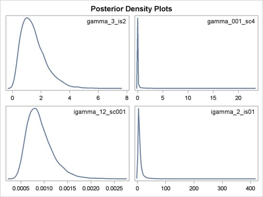
data a;
run;

ods graphics on;
ods select DensityPanel;
proc mcmc data=a stats=none diag=none nmc=10000 outpost=gout
   plots=density seed=1;
   parms gamma_3_is2 gamma_001_sc4 igamma_12_sc001 igamma_2_is01;
   prior gamma_3_is2     ~  gamma(shape=3, iscale=2);
   prior gamma_001_sc4   ~  gamma(shape=0.01, scale=4);
   prior igamma_12_sc001 ~ igamma(shape=12, scale=0.01);
   prior igamma_2_is01   ~ igamma(shape=2, iscale=0.1);
   model general(0);
run;
ods graphics off;

The preceding statements specify four different gamma and inverse gamma distributions with various scale and inverse scale parameter values. The output of kernel density plots of these four prior distributions is shown in Figure 61.19. Note how the X axis scales vary across different distributions.