The GLIMMIX Procedure
-
Overview

-
Getting Started
-
SyntaxPROC GLIMMIX StatementBY StatementCLASS StatementCODE StatementCONTRAST StatementCOVTEST StatementEFFECT StatementESTIMATE StatementFREQ StatementID StatementLSMEANS StatementLSMESTIMATE StatementMODEL StatementNLOPTIONS StatementOUTPUT StatementPARMS StatementRANDOM StatementSLICE StatementSTORE StatementWEIGHT StatementProgramming StatementsUser-Defined Link or Variance Function
-
DetailsGeneralized Linear Models TheoryGeneralized Linear Mixed Models TheoryGLM Mode or GLMM ModeStatistical Inference for Covariance ParametersDegrees of Freedom MethodsEmpirical Covariance (Sandwich) EstimatorsExploring and Comparing Covariance MatricesProcessing by SubjectsRadial Smoothing Based on Mixed ModelsOdds and Odds Ratio EstimationParameterization of Generalized Linear Mixed ModelsResponse-Level Ordering and ReferencingComparing the GLIMMIX and MIXED ProceduresSingly or Doubly Iterative FittingDefault Estimation TechniquesDefault OutputNotes on Output StatisticsODS Table NamesODS Graphics
-
ExamplesBinomial Counts in Randomized BlocksMating Experiment with Crossed Random EffectsSmoothing Disease Rates; Standardized Mortality RatiosQuasi-likelihood Estimation for Proportions with Unknown DistributionJoint Modeling of Binary and Count DataRadial Smoothing of Repeated Measures DataIsotonic Contrasts for Ordered AlternativesAdjusted Covariance Matrices of Fixed EffectsTesting Equality of Covariance and Correlation MatricesMultiple Trends Correspond to Multiple Extrema in Profile LikelihoodsMaximum Likelihood in Proportional Odds Model with Random EffectsFitting a Marginal (GEE-Type) ModelResponse Surface Comparisons with Multiplicity AdjustmentsGeneralized Poisson Mixed Model for Overdispersed Count DataComparing Multiple B-SplinesDiallel Experiment with Multimember Random EffectsLinear Inference Based on Summary DataWeighted Multilevel Model for Survey Data
- References
LSMEANS fixed-effects </ options> ;
The LSMEANS statement computes least squares means (LS-means) of fixed effects. As in the GLM and the MIXED procedures, LS-means
are predicted population margins—that is, they estimate the marginal means over a balanced population. In a sense, LS-means are to unbalanced designs as class
and subclass arithmetic means are to balanced designs. The ![]() matrix constructed to compute them is the same as the
matrix constructed to compute them is the same as the ![]() matrix formed in PROC GLM; however, the standard errors are adjusted for the covariance parameters in the model. Least squares
means computations are not supported for multinomial models.
matrix formed in PROC GLM; however, the standard errors are adjusted for the covariance parameters in the model. Least squares
means computations are not supported for multinomial models.
Each LS-mean is computed as ![]() , where
, where ![]() is the coefficient matrix associated with the least squares mean and
is the coefficient matrix associated with the least squares mean and ![]() is the estimate of the fixed-effects parameter vector. The approximate standard error for the LS-mean is computed as the
square root of
is the estimate of the fixed-effects parameter vector. The approximate standard error for the LS-mean is computed as the
square root of ![]() . The approximate variance matrix of the fixed-effects estimates depends on the estimation method.
. The approximate variance matrix of the fixed-effects estimates depends on the estimation method.
LS-means are constructed on the linked scale—that is, the scale on which the model effects are additive. For example, in a binomial model with logit link, the least squares means are predicted population margins of the logits.
LS-means can be computed for any effect in the MODEL statement that involves only CLASS variables. You can specify multiple effects in one LSMEANS statement or in multiple LSMEANS statements, and all LSMEANS statements
must appear after the MODEL statement. As in the ESTIMATE statement, the ![]() matrix is tested for estimability, and if this test fails, PROC GLIMMIX displays “Non-est” for the LS-means entries.
matrix is tested for estimability, and if this test fails, PROC GLIMMIX displays “Non-est” for the LS-means entries.
Assuming the LS-mean is estimable, PROC GLIMMIX constructs an approximate t test to test the null hypothesis that the associated population quantity equals zero. By default, the denominator degrees of freedom for this test are the same as those displayed for the effect in the “Type III Tests of Fixed Effects” table. If the DDFM=SATTERTHWAITE or DDFM=KENWARDROGER option is specified in the MODEL statement, PROC GLIMMIX determines degrees of freedom separately for each test, unless the DDF= option overrides it for a particular effect. See the DDFM= option for more information. Table 43.8 summarizes options available in the LSMEANS statement. All LSMEANS options are subsequently discussed in alphabetical order.
Table 43.8: LSMEANS Statement Options
|
Option |
Description |
|---|---|
|
Construction and Computation of LS-Means |
|
|
Modifies covariate value in computing LS-means |
|
|
Computes separate margins |
|
|
Requests differences of LS-means |
|
|
Specifies weighting scheme for LS-mean computation as determined by the input data set |
|
|
Tunes estimability checking |
|
|
Partitions F tests (simple effects) |
|
|
Requests simple effects differences |
|
|
Determines the type of simple difference |
|
|
Degrees of Freedom and P-values |
|
|
Determines whether to compute row-wise denominator degrees of freedom with DDFM=SATTERTHWAITE or DDFM=KENWARDROGER |
|
|
Determines the method for multiple comparison adjustment of LS-mean differences |
|
|
Determines the confidence level ( |
|
|
Assigns specific value to degrees of freedom for tests and confidence limits |
|
|
Adjusts multiple comparison p-values further in a step-down fashion |
|
|
Statistical Output |
|
|
Constructs confidence limits for means and or mean differences |
|
|
Displays correlation matrix of LS-means |
|
|
Displays covariance matrix of LS-means |
|
|
Prints the |
|
|
Applies the inverse link transform to the LS-Means (not differences) and produces the standard errors on the inverse linked scale |
|
|
Produces “Lines” display for pairwise LS-mean differences |
|
|
Reports odds of levels of fixed effects if permissible by the link function |
|
|
Reports (simple) differences of least squares means in terms of odds ratios if permissible by the link function |
|
|
Requests ODS statistical graphics of means and mean comparisons |
|
You can specify the following options in the LSMEANS statement after a slash (/).
- ADJDFE=ROW | SOURCE
-
specifies how denominator degrees of freedom are determined when p-values and confidence limits are adjusted for multiple comparisons with the ADJUST= option. When you do not specify the ADJDFE= option, or when you specify ADJDFE=SOURCE, the denominator degrees of freedom for multiplicity-adjusted results are the denominator degrees of freedom for the LS-mean effect in the “Type III Tests of Fixed Effects” table. When you specify ADJDFE=ROW, the denominator degrees of freedom for multiplicity-adjusted results correspond to the degrees of freedom displayed in the
DFcolumn of the “Differences of Least Squares Means” table.The ADJDFE=ROW setting is particularly useful if you want multiplicity adjustments to take into account that denominator degrees of freedom are not constant across LS-mean differences. This can be the case, for example, when the DDFM=SATTERTHWAITE or DDFM=KENWARDROGER degrees-of-freedom method is in effect.
In one-way models with heterogeneous variance, combining certain ADJUST= options with the ADJDFE=ROW option corresponds to particular methods of performing multiplicity adjustments in the presence of heteroscedasticity. For example, the following statements fit a heteroscedastic one-way model and perform Dunnett’s T3 method (Dunnett, 1980), which is based on the studentized maximum modulus (ADJUST=SMM):
proc glimmix;
   class A;
   model y = A / ddfm=satterth;
   random _residual_ / group=A;
   lsmeans A / adjust=smm adjdfe=row;
run;
If you combine the ADJDFE=ROW option with ADJUST=SIDAK, the multiplicity adjustment corresponds to the T2 method of Tamhane (1979), while ADJUST=TUKEY corresponds to the method of Games-Howell (Games and Howell, 1976). Note that ADJUST=TUKEY gives the exact results for the case of fractional degrees of freedom in the one-way model, but it does not take into account that the degrees of freedom are subject to variability. A more conservative method, such as ADJUST=SMM, might protect the overall error rate better.
Unless the ADJUST= option is specified in the LSMEANS statement, the ADJDFE= option has no effect.
-
ADJUST=BON
ADJUST=DUNNETT
ADJUST=NELSON
ADJUST=SCHEFFE
ADJUST=SIDAK
ADJUST=SIMULATE<(simoptions)>
ADJUST=SMM | GT2
ADJUST=TUKEY -
requests a multiple comparison adjustment for the p-values and confidence limits for the differences of LS-means. The adjusted quantities are produced in addition to the unadjusted quantities. By default, PROC GLIMMIX performs all pairwise differences. If you specify ADJUST=DUNNETT, the procedure analyzes all differences with a control level. If you specify ADJUST=NELSON, ANOM differences are taken. The ADJUST= option implies the DIFF option, unless the SLICEDIFF= option is specified.
The BON (Bonferroni) and SIDAK adjustments involve correction factors described in Chapter 44: The GLM Procedure, and Chapter 65: The MULTTEST Procedure; also see Westfall and Young (1993) and Westfall et al. (1999). When you specify ADJUST=TUKEY and your data are unbalanced, PROC GLIMMIX uses the approximation described in Kramer (1956) and identifies the adjustment as “Tukey-Kramer” in the results. Similarly, when you specify ADJUST=DUNNETT or ADJUST=NELSON and the LS-means are correlated, the GLIMMIX procedure uses the factor-analytic covariance approximation described in Hsu (1992) and identifies the adjustment in the results as “Dunnett-Hsu” or “Nelson-Hsu,” respectively. The approximation derives an approximate “effective sample sizes” for which exact critical values are computed. Note that computing the exact adjusted p-values and critical values for unbalanced designs can be computationally intensive, in particular for ADJUST=NELSON. A simulation-based approach, as specified by the ADJUST=SIM option, while nondeterministic, can provide inferences that are sufficiently accurate in much less time. The preceding references also describe the SCHEFFE and SMM adjustments.
Nelson’s adjustment applies only to the analysis of means (Ott, 1967; Nelson, 1982, 1991, 1993), where LS-means are compared against an average LS-mean. It does not apply to all pairwise differences of least squares means, or to slice differences that you specify with the SLICEDIFF= option. See the DIFF=ANOM option for more details regarding the analysis of means with the GLIMMIX procedure.
The SIMULATE adjustment computes adjusted p-values and confidence limits from the simulated distribution of the maximum or maximum absolute value of a multivariate t random vector. All covariance parameters, except the residual scale parameter, are fixed at their estimated values throughout the simulation, potentially resulting in some underdispersion. The simulation estimates q, the true
 quantile, where
  is the confidence coefficient. The default
  is 0.05, and you can change this value with the ALPHA= option in the LSMEANS statement.
The number of samples is set so that the tail area for the simulated q is within
 of with
  % confidence. In equation form,
![\[ \mr {Pr}(|F(\widehat{q})-(1-\alpha )| \leq \gamma ) = 1 - \epsilon \]](images/statug_glimmix0190.png)
where
 is the simulated q and F is the true distribution function of the maximum; see Edwards and Berry (1987) for details. By default, = 0.005 and
  = 0.01, placing the tail area of within 0.005 of 0.95 with 99% confidence. The ACC= and EPS= simoptions reset and , respectively, the NSAMP= simoption sets the sample size directly, and the SEED= simoption specifies an integer used to start the pseudo-random number generator for the simulation. If you do not specify a seed, or
if you specify a value less than or equal to zero, the seed is generated from reading the time of day from the computer clock.
For additional descriptions of these and other simulation options, see the section LSMEANS Statement in Chapter 44: The GLM Procedure.
= 0.01, placing the tail area of within 0.005 of 0.95 with 99% confidence. The ACC= and EPS= simoptions reset and , respectively, the NSAMP= simoption sets the sample size directly, and the SEED= simoption specifies an integer used to start the pseudo-random number generator for the simulation. If you do not specify a seed, or
if you specify a value less than or equal to zero, the seed is generated from reading the time of day from the computer clock.
For additional descriptions of these and other simulation options, see the section LSMEANS Statement in Chapter 44: The GLM Procedure.
If the STEPDOWN option is in effect, the p-values are further adjusted in a step-down fashion. For certain options and data, this adjustment is exact under an iid
 model for the dependent variable, in particular for the following:
-
for ADJUST=DUNNETT when the means are uncorrelated
-
for ADJUST=TUKEY with STEPDOWN(TYPE=LOGICAL) when the means are balanced and uncorrelated.
The first case is a consequence of the nature of the successive step-down hypotheses for comparisons with a control; the second employs an extension of the maximum studentized range distribution appropriate for partition hypotheses (Royen, 1989). Finally, for STEPDOWN(TYPE=FREE), ADJUST=TUKEY employs the Royen (1989) extension in such a way that the resulting p-values are conservative.
-
- ALPHA=number
-
requests that a t-type confidence interval be constructed for each of the LS-means with confidence level 1 – number. The value of number must be between 0 and 1; the default is 0.05.
-
AT variable=value
AT (variable-list)=(value-list)
AT MEANS -
enables you to modify the values of the covariates used in computing LS-means. By default, all covariate effects are set equal to their mean values for computation of standard LS-means. The AT option enables you to assign arbitrary values to the covariates. Additional columns in the output table indicate the values of the covariates.
If there is an effect containing two or more covariates, the AT option sets the effect equal to the product of the individual means rather than the mean of the product (as with standard LS-means calculations). The AT MEANS option sets covariates equal to their mean values (as with standard LS-means) and incorporates this adjustment to crossproducts of covariates.
As an example, consider the following invocation of PROC GLIMMIX:
proc glimmix;
   class A;
   model Y = A x1 x2 x1*x2;
   lsmeans A;
   lsmeans A / at means;
   lsmeans A / at x1=1.2;
   lsmeans A / at (x1 x2)=(1.2 0.3);
run;
For the first two LSMEANS statements, the LS-means coefficient for
x1is (the mean of
 x1) and forx2is (the mean of
 x2). However, for the first LSMEANS statement, the coefficient forx1*x2is , but for the second LSMEANS statement, the coefficient is
  . The third LSMEANS statement sets the coefficient for
 x1equal to 1.2 and leaves it at for x2, and the final LSMEANS statement sets these values to 1.2 and 0.3, respectively.Even if you specify a WEIGHT variable, the unweighted covariate means are used for the covariate coefficients if there is no AT specification. If you specify the AT option, WEIGHT or FREQ variables are taken into account as follows. The weighted covariate means are then used for the covariate coefficients for which no explicit AT values are given, or if you specify AT MEANS. Observations that do not contribute to the analysis because of a missing dependent variable are included in computing the covariate means. You should use the E option in conjunction with the AT option to check that the modified LS-means coefficients are the ones you want.
The AT option is disabled if you specify the BYLEVEL option.
- BYLEVEL
-
requests that separate margins be computed for each level of the LSMEANS effect.
The standard LS-means have equal coefficients across classification effects. The BYLEVEL option changes these coefficients to be proportional to the observed margins. This adjustment is reasonable when you want your inferences to apply to a population that is not necessarily balanced but has the margins observed in the input data set. In this case, the resulting LS-means are actually equal to raw means for fixed-effects models and certain balanced random-effects models, but their estimated standard errors account for the covariance structure that you have specified. If a WEIGHT statement is specified, PROC GLIMMIX uses weighted margins to construct the LS-means coefficients.
If the AT option is specified, the BYLEVEL option disables it.
- CL
-
requests that t-type confidence limits be constructed for each of the LS-means. If DDFM=NONE, then PROC GLIMMIX uses infinite degrees of freedom for this test, essentially computing a z interval. The confidence level is 0.95 by default; this can be changed with the ALPHA= option. If you specify an ADJUST= option, then the confidence limits are adjusted for multiplicity, but if you also specify STEPDOWN, then only p-values are step-down adjusted, not the confidence limits.
- CORR
-
displays the estimated correlation matrix of the least squares means as part of the “Least Squares Means” table.
- COV
-
displays the estimated covariance matrix of the least squares means as part of the “Least Squares Means” table.
- DF=number
-
specifies the degrees of freedom for the t test and confidence limits. The default is the denominator degrees of freedom taken from the “Type III Tests of Fixed Effects” table corresponding to the LS-means effect.
-
DIFF<=difftype>
PDIFF<=difftype> -
requests that differences of the LS-means be displayed. The optional difftype specifies which differences to produce, with possible values ALL, ANOM, CONTROL, CONTROLL, and CONTROLU. The ALL value requests all pairwise differences, and it is the default. The CONTROL difftype requests differences with a control, which, by default, is the first level of each of the specified LSMEANS effects.
The ANOM value requests differences between each LS-mean and the average LS-mean, as in the analysis of means (Ott, 1967). The average is computed as a weighted mean of the LS-means, the weights being inversely proportional to the diagonal entries of the
![\[ \bL \left(\bX ’\bX \right)^{-} \bL ’ \]](images/statug_glimmix0197.png)
matrix. If LS-means are nonestimable, this design-based weighted mean is replaced with an equally weighted mean. Note that the ANOM procedure in SAS/QC software implements both tables and graphics for the analysis of means with a variety of response types. For one-way designs and normal data with identity link, the DIFF=ANOM computations are equivalent to the results of PROC ANOM. If the LS-means being compared are uncorrelated, exact adjusted p-values and critical values for confidence limits can be computed in the analysis of means; see Nelson (1982, 1991, 1993); Guirguis and Tobias (2004) as well as the documentation for the ADJUST=NELSON option.
To specify which levels of the effects are the controls, list the quoted formatted values in parentheses after the CONTROL keyword. For example, if the effects
A,B, andCare classification variables, each having two levels, 1 and 2, the following LSMEANS statement specifies the (1,2) level ofA*Band the (2,1) level ofB*Cas controls:lsmeans A*B B*C / diff=control('1' '2' '2' '1');For multiple effects, the results depend upon the order of the list, and so you should check the output to make sure that the controls are correct.
Two-tailed tests and confidence limits are associated with the CONTROL difftype. For one-tailed results, use either the CONTROLL or CONTROLU difftype. The CONTROLL difftype tests whether the noncontrol levels are significantly smaller than the control; the upper confidence limits for the control minus the noncontrol levels are considered to be infinity and are displayed as missing. Conversely, the CONTROLU difftype tests whether the noncontrol levels are significantly larger than the control; the upper confidence limits for the noncontrol levels minus the control are considered to be infinity and are displayed as missing.
If you want to perform multiple comparison adjustments on the differences of LS-means, you must specify the ADJUST= option.
The differences of the LS-means are displayed in a table titled “Differences of Least Squares Means.”
- E
-
requests that the
 matrix coefficients for the LSMEANS effects
be displayed.
matrix coefficients for the LSMEANS effects
be displayed.
- ILINK
-
requests that estimates and their standard errors in the “Least Squares Means” table also be reported on the scale of the mean (the inverse linked scale). The ILINK option is specific to an LSMEANS statement. If you also specify the CL option, the GLIMMIX procedure computes confidence intervals for the predicted means by applying the inverse link transform to the confidence limits on the linked (linear) scale. Standard errors on the inverse linked scale are computed by the delta method.
The GLIMMIX procedure applies the inverse link transform to the LS-mean reported in the
Estimatecolumn. In a logistic model, for example, this implies that the value reported as the inversely linked estimate corresponds to a predicted probability that is based on an average estimable function (the estimable function that produces the LS-mean on the linear scale). To compute average predicted probabilities, you can average the results from applying the ILINK option in the ESTIMATE statement for suitably chosen estimable functions. - LINES
-
presents results of comparisons between all pairs of least squares means by listing the means in descending order and indicating nonsignificant subsets by line segments beside the corresponding LS-means. When all differences have the same variance, these comparison lines are guaranteed to accurately reflect the inferences based on the corresponding tests, made by comparing the respective p-values to the value of the ALPHA= option (0.05 by default). However, equal variances might not be the case for differences between LS-means. If the variances are not all the same, then the comparison lines might be conservative, in the sense that if you base your inferences on the lines alone, you will detect fewer significant differences than the tests indicate. If there are any such differences, PROC GLIMMIX lists the pairs of means that are inferred to be significantly different by the tests but not by the comparison lines. Note, however, that in many cases, even though the variances are unequal, they are similar enough that the comparison lines accurately reflect the test inferences.
- ODDS
-
requests that in models with logit, cumulative logit, and generalized logit link function the odds of the levels of the fixed effects are reported. If you specify the CL or ALPHA= option, confidence intervals for the odds are also computed. See the section Odds and Odds Ratio Estimation for further details about computation and interpretation of odds and odds ratios with the GLIMMIX procedure.
-
ODDSRATIO
OR -
requests that LS-mean differences (DIFF, ADJUST= options) and simple effect comparisons (SLICEDIFF option) are also reported in terms of odds ratios. The ODDSRATIO option is ignored unless you use either the logit, cumulative logit, or generalized logit link function. If you specify the CL or ALPHA= option, confidence intervals for the odds ratios are also computed. These intervals are adjusted for multiplicity when you specify the ADJUST= option. See the section Odds and Odds Ratio Estimation for further details about computation and interpretation of odds and odds ratios with the GLIMMIX procedure.
-
OBSMARGINS
OM -
specifies a potentially different weighting scheme for the computation of LS-means coefficients. The standard LS-means have equal coefficients across classification effects; however, the OM option changes these coefficients to be proportional to those found in the input data set. This adjustment is reasonable when you want your inferences to apply to a population that is not necessarily balanced but has the margins observed in your data.
In computing the observed margins, PROC GLIMMIX uses all observations for which there are no missing or invalid independent variables, including those for which there are missing dependent variables. Also, if you use a WEIGHT statement, PROC GLIMMIX computes weighted margins to construct the LS-means coefficients. If your data are balanced, the LS-means are unchanged by the OM option.
The BYLEVEL option modifies the observed-margins LS-means. Instead of computing the margins across all of the input data set, PROC GLIMMIX computes separate margins for each level of the LSMEANS effect in question. In this case the resulting LS-means are actually equal to raw means for fixed-effects models and certain balanced random-effects models, but their estimated standard errors account for the covariance structure that you have specified.
You can use the E option in conjunction with either the OM or BYLEVEL option to check that the modified LS-means coefficients are the ones you want. It is possible that the modified LS-means are not estimable when the standard ones are estimable, or vice versa.
- PDIFF
-
is the same as the DIFF option.
-
PLOT | PLOTS<=plot-request<(options)>>
PLOT | PLOTS<=(plot-request<(options)> <…plot-request<(options)> >)> -
creates least squares means related graphs when ODS Graphics has been enabled and the plot request does not conflict with other options in the LSMEANS statement. For general information about ODS Graphics, see Chapter 21: Statistical Graphics Using ODS. For examples of the basic statistical graphics for least squares means and aspects of their computation and interpretation, see the section Graphics for LS-Mean Comparisons in this chapter.
The options for a specific plot request (and their suboptions) of the LSMEANS statement include those for the PLOTS= option in the PROC GLIMMIX statement. You can specify classification effects in the MEANPLOT request of the LSMEANS statement to control the display of interaction means with the PLOTBY= and SLICEBY= suboptions; these are not available in the PLOTS= option in the PROC GLIMMIX statement. Options specified in the LSMEANS statement override those in the PLOTS= option in the PROC GLIMMIX statement.
The available options and suboptions are as follows.
When LS-mean calculations are adjusted for multiplicity by using the ADJUST= option, the plots are adjusted accordingly.
- SINGULAR=number
-
tunes the estimability checking as documented for the CONTRAST statement.
- SLICE=fixed-effect | (fixed-effects)
-
specifies effects by which to partition interaction LSMEANS effects. This can produce what are known as tests of simple effects (Winer, 1971). For example, suppose that
A*Bis significant, and you want to test the effect ofAfor each level ofB. The appropriate LSMEANS statement islsmeans A*B / slice=B;
This statement tests for the simple main effects of
AforB, which are calculated by extracting the appropriate rows from the coefficient matrix for theA*BLS-means and by using them to form an F test.The SLICE option produces F tests that test the simultaneous equality of cell means at a fixed level of the slice effect (Schabenberger, Gregoire, and Kong, 2000). You can request differences of the least squares means while holding one or more factors at a fixed level with the SLICEDIFF= option.
The SLICE option produces a table titled “Tests of Effect Slices.”
-
SLICEDIFF=fixed-effect | (fixed-effects)
SIMPLEDIFF=fixed-effect | (fixed-effects) -
requests that differences of simple effects be constructed and tested against zero. Whereas the SLICE option extracts multiple rows of the coefficient matrix and forms an F test, the SLICEDIFF option tests pairwise differences of these rows. This enables you to perform multiple comparisons among the levels of one factor at a fixed level of the other factor. For example, assume that, in a balanced design, factors
AandBhave a = 4 and b = 3 levels, respectively. Consider the following statements:proc glimmix; class a b; model y = a b a*b; lsmeans a*b / slice=a; lsmeans a*b / slicediff=a; run;
The first LSMEANS statement produces four F tests, one per level of
A. The first of these tests is constructed by extracting the three rows corresponding to the first level ofAfrom the coefficient matrix for theA*Binteraction. Call this matrix and its rows
  ,
,  , and
, and  . The SLICE tests the two-degrees-of-freedom hypothesis
![\[ H\colon \left\{ \begin{array}{c} \left( \mb {l}^{(1)}_{a1} - \mb {l}^{(2)}_{a1}\right) \bbeta = 0 \\ \left( \mb {l}^{(1)}_{a1} - \mb {l}^{(3)}_{a1}\right) \bbeta = 0 \end{array} \right. \]](images/statug_glimmix0202.png)
In a balanced design, where
 denotes the mean response if
 Ais at level i andBis at level j, this hypothesis is equivalent to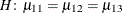 . The SLICEDIFF option considers the three rows of in turn and performs tests of the difference between pairs of rows. How these differences are constructed depends on the
SLICEDIFFTYPE= option. By default, all pairwise differences within the subset of are considered; in the example this corresponds to tests of the form
. The SLICEDIFF option considers the three rows of in turn and performs tests of the difference between pairs of rows. How these differences are constructed depends on the
SLICEDIFFTYPE= option. By default, all pairwise differences within the subset of are considered; in the example this corresponds to tests of the form
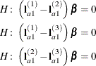
In the example, with a = 4 and b = 3, the second LSMEANS statement produces four sets of least squares means differences. Within each set, factor
Ais held fixed at a particular level and each set consists of three comparisons.When the ADJUST= option is specified, the GLIMMIX procedure also adjusts the tests for multiplicity. The adjustment is based on the number of comparisons within each level of the SLICEDIFF= effect; see the SLICEDIFFTYPE= option. The Nelson adjustment is not available for slice differences.
-
SLICEDIFFTYPE<=difftype>
SIMPLEDIFFTYPE<=difftype> -
determines the type of simple effect differences produced with the SLICEDIFF= option.
The possible values for the difftype are ALL, CONTROL, CONTROLL, and CONTROLU. The difftype ALL requests all simple effects differences, and it is the default. The difftype CONTROL requests the differences with a control, which, by default, is the first level of each of the specified LSMEANS effects.
To specify which levels of the effects are the controls, list the quoted formatted values in parentheses after the keyword CONTROL. For example, if the effects
A,B, andCare classification variables, each having three levels (1, 2, and 3), the following LSMEANS statement specifies the (1,3) level ofA*Bas the control:lsmeans A*B / slicediff=(A B) slicedifftype=control('1' '3');This LSMEANS statement first produces simple effects differences holding the levels of
Afixed, and then it produces simple effects differences holding the levels ofBfixed. In the former case, level ’3’ ofBserves as the control level. In the latter case, level ’1’ ofAserves as the control.For multiple effects, the results depend upon the order of the list, and so you should check the output to make sure that the controls are correct.
Two-tailed tests and confidence limits are associated with the CONTROL difftype. For one-tailed results, use either the CONTROLL or CONTROLU difftype. The CONTROLL difftype tests whether the noncontrol levels are significantly smaller than the control; the upper confidence limits for the control minus the noncontrol levels are considered to be infinity and are displayed as missing. Conversely, the CONTROLU difftype tests whether the noncontrol levels are significantly larger than the control; the upper confidence limits for the noncontrol levels minus the control are considered to be infinity and are displayed as missing.
- STEPDOWN<(step-down options)>
-
requests that multiple comparison adjustments for the p-values of LS-mean differences be further adjusted in a step-down fashion. Step-down methods increase the power of multiple comparisons by taking advantage of the fact that a p-value will never be declared significant unless all smaller p-values are also declared significant. Note that the STEPDOWN adjustment combined with ADJUST=BON corresponds to the methods of Holm (1979) and “Method 2” of Shaffer (1986); this is the default. Using step-down-adjusted p-values combined with ADJUST=SIMULATE corresponds to the method of Westfall (1997).
If the degrees-of-freedom method is DDFM=KENWARDROGER or DDFM=SATTERTHWAITE, then step-down-adjusted p-values are produced only if the ADJDFE=ROW option is in effect.
Also, STEPDOWN affects only p-values, not confidence limits. For ADJUST=SIMULATE, the generalized least squares hybrid approach of Westfall (1997) is employed to increase Monte Carlo accuracy.
You can specify the following step-down options in parentheses: