The GLIMMIX Procedure
-
Overview

-
Getting Started
-
SyntaxPROC GLIMMIX StatementBY StatementCLASS StatementCODE StatementCONTRAST StatementCOVTEST StatementEFFECT StatementESTIMATE StatementFREQ StatementID StatementLSMEANS StatementLSMESTIMATE StatementMODEL StatementNLOPTIONS StatementOUTPUT StatementPARMS StatementRANDOM StatementSLICE StatementSTORE StatementWEIGHT StatementProgramming StatementsUser-Defined Link or Variance Function
-
DetailsGeneralized Linear Models TheoryGeneralized Linear Mixed Models TheoryGLM Mode or GLMM ModeStatistical Inference for Covariance ParametersDegrees of Freedom MethodsEmpirical Covariance (Sandwich) EstimatorsExploring and Comparing Covariance MatricesProcessing by SubjectsRadial Smoothing Based on Mixed ModelsOdds and Odds Ratio EstimationParameterization of Generalized Linear Mixed ModelsResponse-Level Ordering and ReferencingComparing the GLIMMIX and MIXED ProceduresSingly or Doubly Iterative FittingDefault Estimation TechniquesDefault OutputNotes on Output StatisticsODS Table NamesODS Graphics
-
ExamplesBinomial Counts in Randomized BlocksMating Experiment with Crossed Random EffectsSmoothing Disease Rates; Standardized Mortality RatiosQuasi-likelihood Estimation for Proportions with Unknown DistributionJoint Modeling of Binary and Count DataRadial Smoothing of Repeated Measures DataIsotonic Contrasts for Ordered AlternativesAdjusted Covariance Matrices of Fixed EffectsTesting Equality of Covariance and Correlation MatricesMultiple Trends Correspond to Multiple Extrema in Profile LikelihoodsMaximum Likelihood in Proportional Odds Model with Random EffectsFitting a Marginal (GEE-Type) ModelResponse Surface Comparisons with Multiplicity AdjustmentsGeneralized Poisson Mixed Model for Overdispersed Count DataComparing Multiple B-SplinesDiallel Experiment with Multimember Random EffectsLinear Inference Based on Summary DataWeighted Multilevel Model for Survey Data
- References
The GLIMMIX procedure has facilities for multiplicity-adjusted inference through the ADJUST= and STEPDOWN options in the ESTIMATE, LSMEANS, and LSMESTIMATE statements. You can employ these facilities to test linear hypotheses among parameters even in situations where the quantities were obtained outside the GLIMMIX procedure. This example demonstrates the process. The basic idea is to prepare a data set containing the estimates of interest and a data set containing their covariance matrix. These are then passed to the GLIMMIX procedure, preventing updating of the parameters, essentially moving directly into the post-processing stage as if estimates with this covariance matrix had been produced by the GLIMMIX procedure.
The final documentation example in Chapter 67: The NLIN Procedure, discusses a nonlinear first-order compartment pharmacokinetic model for theophylline concentration. The data are derived by collapsing and averaging the subject-specific data from Pinheiro and Bates (1995) in a particular—yet unimportant—way that leads to two groups for comparisons. The following DATA step creates these data:
data theop;
   input time dose conc @@;
   if (dose = 4) then group=1; else group=2;
   datalines;
 0.00   4  0.1633  0.25   4   2.045
 0.27   4     4.4  0.30   4    7.37
 0.35   4    1.89  0.37   4    2.89
 0.50   4    3.96  0.57   4    6.57
 0.58   4     6.9  0.60   4     4.6
 0.63   4    9.03  0.77   4    5.22
 1.00   4    7.82  1.02   4   7.305
 1.05   4    7.14  1.07   4     8.6
 1.12   4    10.5  2.00   4    9.72
 2.02   4    7.93  2.05   4    7.83
 2.13   4    8.38  3.50   4    7.54
 3.52   4    9.75  3.53   4    5.66
 3.55   4   10.21  3.62   4     7.5
 3.82   4    8.58  5.02   4   6.275
 5.05   4    9.18  5.07   4    8.57
 5.08   4     6.2  5.10   4    8.36
 7.02   4    5.78  7.03   4    7.47
 7.07   4   5.945  7.08   4    8.02
 7.17   4    4.24  8.80   4    4.11
 9.00   4     4.9  9.02   4    5.33
 9.03   4    6.11  9.05   4    6.89
 9.38   4    7.14 11.60   4    3.16
11.98   4    4.19 12.05   4    4.57
12.10   4    5.68 12.12   4    5.94
12.15   4     3.7 23.70   4    2.42
24.15   4    1.17 24.17   4    1.05
24.37   4    3.28 24.43   4    1.12
24.65   4    1.15  0.00   5   0.025
 0.25   5    2.92  0.27   5   1.505
 0.30   5    2.02  0.50   5   4.795
 0.52   5    5.53  0.58   5    3.08
 0.98   5   7.655  1.00   5   9.855
 1.02   5    5.02  1.15   5    6.44
 1.92   5    8.33  1.98   5    6.81
 2.02   5  7.8233  2.03   5    6.32
 3.48   5    7.09  3.50   5   7.795
 3.53   5    6.59  3.57   5    5.53
 3.60   5    5.87  5.00   5     5.8
 5.02   5  6.2867  5.05   5    5.88
 6.98   5    5.25  7.00   5    4.02
 7.02   5    7.09  7.03   5   4.925
 7.15   5    4.73  9.00   5    4.47
 9.03   5    3.62  9.07   5    4.57
 9.10   5     5.9  9.22   5    3.46
12.00   5    3.69 12.05   5    3.53
12.10   5    2.89 12.12   5    2.69
23.85   5    0.92 24.08   5    0.86
24.12   5    1.25 24.22   5    1.15
24.30   5     0.9 24.35   5    1.57
;
In terms of two fixed treatment groups, the nonlinear model for these data can be written as
where ![]() is the observed concentration in group i at time t, D is the dose of theophylline,
is the observed concentration in group i at time t, D is the dose of theophylline, ![]() is the elimination rate constant in group i,
is the elimination rate constant in group i, ![]() is the absorption rate in group i,
is the absorption rate in group i, ![]() is the clearance in group i, and
is the clearance in group i, and ![]() denotes the model error. Because the rates and the clearance must be positive, you can parameterize the model in terms of
log rates and the log clearance:
denotes the model error. Because the rates and the clearance must be positive, you can parameterize the model in terms of
log rates and the log clearance:

In this parameterization the model contains six parameters, and the rates and clearance vary by group. The following PROC NLIN statements fit the model and obtain the group-specific parameter estimates:
proc nlin data=theop outest=cov;
   parms beta1_1=-3.22 beta2_1=0.47 beta3_1=-2.45
         beta1_2=-3.22 beta2_2=0.47 beta3_2=-2.45;
   if (group=1) then do;
      cl   = exp(beta1_1);
      ka   = exp(beta2_1);
      ke   = exp(beta3_1);
   end; else do;
      cl   = exp(beta1_2);
      ka   = exp(beta2_2);
      ke   = exp(beta3_2);
   end;
   mean = dose*ke*ka*(exp(-ke*time)-exp(-ka*time))/cl/(ka-ke);
   model conc = mean;
   ods output ParameterEstimates=ests;
run;
The conditional programming statements determine the clearance, elimination, and absorption rates depending on the value of
the group variable. The OUTEST= option in the PROC NLIN statement saves estimates and their covariance matrix to the data set cov. The ODS OUTPUT statement saves the “Parameter Estimates” table to the data set ests.
Output 43.17.1 displays the analysis of variance table and the parameter estimates from this NLIN run. Note that the confidence levels in the “Parameter Estimates” table are based on 92 degrees of freedom, corresponding to the residual degrees of freedom in the analysis of variance table.
Output 43.17.1: Analysis of Variance and Parameter Estimates for Nonlinear Model
| Note: | An intercept was not specified for this model. |
| Source | DF | Sum of Squares | Mean Square | F Value | Approx Pr > F |
|---|---|---|---|---|---|
| Model | 6 | 3247.9 | 541.3 | 358.56 | <.0001 |
| Error | 92 | 138.9 | 1.5097 | ||
| Uncorrected Total | 98 | 3386.8 |
| Parameter | Estimate | Approx Std Error |
Approximate 95% Confidence Limits |
|
|---|---|---|---|---|
| beta1_1 | -3.5671 | 0.0864 | -3.7387 | -3.3956 |
| beta2_1 | 0.4421 | 0.1349 | 0.1742 | 0.7101 |
| beta3_1 | -2.6230 | 0.1265 | -2.8742 | -2.3718 |
| beta1_2 | -3.0111 | 0.1061 | -3.2219 | -2.8003 |
| beta2_2 | 0.3977 | 0.1987 | 0.00305 | 0.7924 |
| beta3_2 | -2.4442 | 0.1618 | -2.7655 | -2.1229 |
The following DATA step extracts the part of the cov data set that contains the covariance matrix of the parameter estimates in Output 43.17.1 and renames the variables as Col1–Col6. Output 43.17.2 shows the result of the DATA step.
data covb;
   set cov(where=(_type_='COVB'));
   rename beta1_1=col1 beta2_1=col2 beta3_1=col3
          beta1_2=col4 beta2_2=col5 beta3_2=col6;
   row = _n_;
   Parm = 1;
   keep parm row beta:;
run;
proc print data=covb;
run;
Output 43.17.2: Covariance Matrix of NLIN Parameter Estimates
| Obs | col1 | col2 | col3 | col4 | col5 | col6 | row | Parm |
|---|---|---|---|---|---|---|---|---|
| 1 | 0.007462 | -0.005222 | 0.010234 | 0.000000 | 0.000000 | 0.000000 | 1 | 1 |
| 2 | -0.005222 | 0.018197 | -0.010590 | 0.000000 | 0.000000 | 0.000000 | 2 | 1 |
| 3 | 0.010234 | -0.010590 | 0.015999 | 0.000000 | 0.000000 | 0.000000 | 3 | 1 |
| 4 | 0.000000 | 0.000000 | 0.000000 | 0.011261 | -0.009096 | 0.015785 | 4 | 1 |
| 5 | 0.000000 | 0.000000 | 0.000000 | -0.009096 | 0.039487 | -0.019996 | 5 | 1 |
| 6 | 0.000000 | 0.000000 | 0.000000 | 0.015785 | -0.019996 | 0.026172 | 6 | 1 |
The reason for this transformation of the data is to use the resulting data set to define a covariance structure in PROC GLIMMIX. The following statements reconstitute a model in which the parameter estimates from PROC NLIN are the observations and in which the covariance matrix of the “observations” matches the covariance matrix of the NLIN parameter estimates:
proc glimmix data=ests order=data;
   class Parameter;
   model Estimate = Parameter / noint df=92 s;
   random _residual_ / type=lin(1) ldata=covb v;
   parms (1) / noiter;
   lsmeans parameter / cl;
   lsmestimate Parameter
               'beta1 eq. across groups' 1 0 0 -1,
               'beta2 eq. across groups' 0 1 0  0 -1,
               'beta3 eq. across groups' 0 0 1  0  0  -1 /
               adjust=bon stepdown ftest(label='Homogeneity');
run;
In other words, you are using PROC GLIMMIX to set up a linear statistical model
where the covariance matrix ![]() is given by
is given by
![\[ \mb {A} = \left[ \begin{array}{llllll} \mbox{\phantom{--}} 0.007 & -0.005 & \mbox{\phantom{--}} 0.010 & \mbox{\phantom{--}} 0 & \mbox{\phantom{--}} 0 & \mbox{\phantom{--}} 0 \\ -0.005 & \mbox{\phantom{--}} 0.018 & -0.011 & \mbox{\phantom{--}} 0 & \mbox{\phantom{--}} 0 & \mbox{\phantom{--}} 0 \\ \mbox{\phantom{--}} 0.010 & -0.011 & \mbox{\phantom{--}} 0.016 & \mbox{\phantom{--}} 0 & \mbox{\phantom{--}} 0 & \mbox{\phantom{--}} 0 \\ \mbox{\phantom{--}} 0 & \mbox{\phantom{--}} 0 & \mbox{\phantom{--}} 0 & \mbox{\phantom{--}} 0.011 & -0.009 & \mbox{\phantom{--}} 0.016 \\ \mbox{\phantom{--}} 0 & \mbox{\phantom{--}} 0 & \mbox{\phantom{--}} 0 & -0.009 & \mbox{\phantom{--}} 0.039 & -0.019 \\ \mbox{\phantom{--}} 0 & \mbox{\phantom{--}} 0 & \mbox{\phantom{--}} 0 & \mbox{\phantom{--}} 0.016 & -0.019 & \mbox{\phantom{--}} 0.026 \\ \end{array}\right]\\ \]](images/statug_glimmix1102.png)
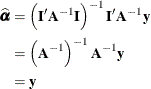
The generalized least squares estimate for ![]() in this saturated model reproduces the observations:
in this saturated model reproduces the observations:
The ORDER=DATA option in the PROC GLIMMIX statement requests that the sort order of the Parameter variable be identical to the order in which it appeared in the “Parameter Estimates” table of the NLIN procedure (Output 43.17.1). The MODEL statement uses the Estimate and Parameter variables from that table to form a model in which the ![]() matrix is the identity; hence the NOINT option. The DF=92 option sets the degrees of freedom equal to the value used in the NLIN procedure. The RANDOM statement specifies a linear covariance structure with a single component and supplies the values for the structure through
the LDATA= data set. This structure models the covariance matrix as
matrix is the identity; hence the NOINT option. The DF=92 option sets the degrees of freedom equal to the value used in the NLIN procedure. The RANDOM statement specifies a linear covariance structure with a single component and supplies the values for the structure through
the LDATA= data set. This structure models the covariance matrix as ![]() , where the
, where the ![]() matrix is given previously. Essentially, the TYPE=LIN(1) structure forces an unstructured covariance matrix onto the data. To make this work, the parameter
matrix is given previously. Essentially, the TYPE=LIN(1) structure forces an unstructured covariance matrix onto the data. To make this work, the parameter ![]() is held fixed at 1 in the PARMS statement.
is held fixed at 1 in the PARMS statement.
Output 43.17.3 displays the parameter estimates and least squares means for this model. Note that estimates and least squares means are
identical, since the ![]() matrix is the identity. Also, the confidence limits agree with the values reported by PROC NLIN (see Output 43.17.1).
matrix is the identity. Also, the confidence limits agree with the values reported by PROC NLIN (see Output 43.17.1).
Output 43.17.3: Parameter Estimates and LS-Means from Summary Data
| Solutions for Fixed Effects | ||||||
|---|---|---|---|---|---|---|
| Effect | Parameter | Estimate | Standard Error | DF | t Value | Pr > |t| |
| Parameter | beta1_1 | -3.5671 | 0.08638 | 92 | -41.29 | <.0001 |
| Parameter | beta2_1 | 0.4421 | 0.1349 | 92 | 3.28 | 0.0015 |
| Parameter | beta3_1 | -2.6230 | 0.1265 | 92 | -20.74 | <.0001 |
| Parameter | beta1_2 | -3.0111 | 0.1061 | 92 | -28.37 | <.0001 |
| Parameter | beta2_2 | 0.3977 | 0.1987 | 92 | 2.00 | 0.0483 |
| Parameter | beta3_2 | -2.4442 | 0.1618 | 92 | -15.11 | <.0001 |
| Parameter Least Squares Means | ||||||||
|---|---|---|---|---|---|---|---|---|
| Parameter | Estimate | Standard Error | DF | t Value | Pr > |t| | Alpha | Lower | Upper |
| beta1_1 | -3.5671 | 0.08638 | 92 | -41.29 | <.0001 | 0.05 | -3.7387 | -3.3956 |
| beta2_1 | 0.4421 | 0.1349 | 92 | 3.28 | 0.0015 | 0.05 | 0.1742 | 0.7101 |
| beta3_1 | -2.6230 | 0.1265 | 92 | -20.74 | <.0001 | 0.05 | -2.8742 | -2.3718 |
| beta1_2 | -3.0111 | 0.1061 | 92 | -28.37 | <.0001 | 0.05 | -3.2219 | -2.8003 |
| beta2_2 | 0.3977 | 0.1987 | 92 | 2.00 | 0.0483 | 0.05 | 0.003050 | 0.7924 |
| beta3_2 | -2.4442 | 0.1618 | 92 | -15.11 | <.0001 | 0.05 | -2.7655 | -2.1229 |
The (marginal) covariance matrix of the data is shown in Output 43.17.4 to confirm that it matches the ![]() matrix given earlier.
matrix given earlier.
Output 43.17.4: R-Side Covariance Matrix
| Estimated V Matrix for Subject 1 | ||||||
|---|---|---|---|---|---|---|
| Row | Col1 | Col2 | Col3 | Col4 | Col5 | Col6 |
| 1 | 0.007462 | -0.00522 | 0.01023 | |||
| 2 | -0.00522 | 0.01820 | -0.01059 | |||
| 3 | 0.01023 | -0.01059 | 0.01600 | |||
| 4 | 0.01126 | -0.00910 | 0.01579 | |||
| 5 | -0.00910 | 0.03949 | -0.02000 | |||
| 6 | 0.01579 | -0.02000 | 0.02617 | |||
The LSMESTIMATE statement specifies three linear functions. These set equal the ![]() parameters from the groups. The step-down Bonferroni adjustment requests a multiplicity adjustment for the family of three
tests. The FTEST option requests a joint test of the three estimable functions; it is a global test of parameter homogeneity across groups.
parameters from the groups. The step-down Bonferroni adjustment requests a multiplicity adjustment for the family of three
tests. The FTEST option requests a joint test of the three estimable functions; it is a global test of parameter homogeneity across groups.
Output 43.17.5 displays the result from the LSMESTIMATE statement. The joint test is highly significant (F = 30.52, p < 0.0001). From the p-values associated with the individual rows of the estimates, you can see that the lack of homogeneity is due to group differences
for ![]() , the log clearance.
, the log clearance.
Output 43.17.5: Test of Parameter Homogeneity across Groups
| Least Squares Means Estimates Adjustment for Multiplicity: Holm |
|||||||
|---|---|---|---|---|---|---|---|
| Effect | Label | Estimate | Standard Error | DF | t Value | Pr > |t| | Adj P |
| Parameter | beta1 eq. across groups | -0.5560 | 0.1368 | 92 | -4.06 | 0.0001 | 0.0003 |
| Parameter | beta2 eq. across groups | 0.04443 | 0.2402 | 92 | 0.18 | 0.8537 | 0.8537 |
| Parameter | beta3 eq. across groups | -0.1788 | 0.2054 | 92 | -0.87 | 0.3862 | 0.7725 |
| F Test for Least Squares Means Estimates | ||||
|---|---|---|---|---|
| Label | Num DF | Den DF | F Value | Pr > F |
| Homogeneity | 3 | 92 | 30.52 | <.0001 |
An alternative method of setting up this model is given by the following statements, where the data set pdata contains the covariance parameters:
random _residual_ / type=un;
parms / pdata=pdata noiter
The following DATA step creates an appropriate PDATA= data set from the data set covb, which was constructed earlier:
data pdata;
   set covb;
   array col{6};
   do i=1 to _n_;
      estimate = col{i};
      output;
   end;
   keep estimate;
run;