The GLIMMIX Procedure
-
Overview

-
Getting Started
-
SyntaxPROC GLIMMIX StatementBY StatementCLASS StatementCODE StatementCONTRAST StatementCOVTEST StatementEFFECT StatementESTIMATE StatementFREQ StatementID StatementLSMEANS StatementLSMESTIMATE StatementMODEL StatementNLOPTIONS StatementOUTPUT StatementPARMS StatementRANDOM StatementSLICE StatementSTORE StatementWEIGHT StatementProgramming StatementsUser-Defined Link or Variance Function
-
DetailsGeneralized Linear Models TheoryGeneralized Linear Mixed Models TheoryGLM Mode or GLMM ModeStatistical Inference for Covariance ParametersDegrees of Freedom MethodsEmpirical Covariance (Sandwich) EstimatorsExploring and Comparing Covariance MatricesProcessing by SubjectsRadial Smoothing Based on Mixed ModelsOdds and Odds Ratio EstimationParameterization of Generalized Linear Mixed ModelsResponse-Level Ordering and ReferencingComparing the GLIMMIX and MIXED ProceduresSingly or Doubly Iterative FittingDefault Estimation TechniquesDefault OutputNotes on Output StatisticsODS Table NamesODS Graphics
-
ExamplesBinomial Counts in Randomized BlocksMating Experiment with Crossed Random EffectsSmoothing Disease Rates; Standardized Mortality RatiosQuasi-likelihood Estimation for Proportions with Unknown DistributionJoint Modeling of Binary and Count DataRadial Smoothing of Repeated Measures DataIsotonic Contrasts for Ordered AlternativesAdjusted Covariance Matrices of Fixed EffectsTesting Equality of Covariance and Correlation MatricesMultiple Trends Correspond to Multiple Extrema in Profile LikelihoodsMaximum Likelihood in Proportional Odds Model with Random EffectsFitting a Marginal (GEE-Type) ModelResponse Surface Comparisons with Multiplicity AdjustmentsGeneralized Poisson Mixed Model for Overdispersed Count DataComparing Multiple B-SplinesDiallel Experiment with Multimember Random EffectsLinear Inference Based on Summary DataWeighted Multilevel Model for Survey Data
- References
Koch et al. (1990) present data for a multicenter clinical trial testing the efficacy of a respiratory drug in patients with respiratory disease.
Within each of two centers, patients were randomly assigned to a placebo (P) or an active (A) treatment. Prior to treatment
and at four follow-up visits, patient status was recorded in one of five ordered categories (0=terrible, 1=poor, …, 4=excellent).
The following DATA step creates the SAS data set clinical for this study.
data Clinical;
   do Center =   1,  2;
      do Gender = 'F','M';
         do Drug   = 'A','P';
            input nPatient @@;
            do iPatient = 1 to nPatient;
               input ID Age (t0-t4) (1.) @@;
               output;
            end;
         end;
      end;
   end;
   datalines;
 2  53 32 12242  18 47 22344
 5   5 13 44444  19 31 21022  25 35 10000  28 36 23322
    36 45 22221
25  54 11 44442  12 14 23332  51 15 02333  20 20 33231
    16 22 12223  50 22 21344   3 23 33443  32 23 23444
    56 25 23323  35 26 12232  26 26 22222  21 26 24142
     8 28 12212  30 28 00121  33 30 33442  11 30 34443
    42 31 12311   9 31 33444  37 31 02321  23 32 34433
     6 34 11211  22 46 43434  24 48 23202  38 50 22222
    48 57 33434
24  43 13 34444  41 14 22123  34 15 22332  29 19 23300
    15 20 44444  13 23 33111  27 23 44244  55 24 34443
    17 25 11222  45 26 24243  40 26 12122  44 27 12212
    49 27 33433  39 23 21111   2 28 20000  14 30 10000
    31 37 10000  10 37 32332   7 43 23244  52 43 11132
     4 44 34342   1 46 22222  46 49 22222  47 63 22222
 4  30 37 13444  52 39 23444  23 60 44334  54 63 44444
12  28 31 34444   5 32 32234  21 36 33213  50 38 12000
     1 39 12112  48 39 32300   7 44 34444  38 47 23323
     8 48 22100  11 48 22222   4 51 34244  17 58 14220
23  12 13 44444  10 14 14444  27 19 33233  47 20 24443
    16 20 21100  29 21 33444  20 24 44444  25 25 34331
    15 25 34433   2 25 22444   9 26 23444  49 28 23221
    55 31 44444  43 34 24424  26 35 44444  14 37 43224
    36 41 34434  51 43 33442  37 52 12122  19 55 44444
    32 55 22331   3 58 44444  53 68 23334
16  39 11 34444  40 14 21232  24 15 32233  41 15 43334
    33 19 42233  34 20 32444  13 20 14444  45 33 33323
    22 36 24334  18 38 43000  35 42 32222  44 43 21000
     6 45 34212  46 48 44000  31 52 23434  42 66 33344
;
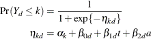
Westfall and Tobias (2007) define as the measure of efficacy the average of the ratings at the final two visits and model this average as a function
of drug, baseline assessment score, and age. Hence, in their model, the expected efficacy for drug ![]() can be written as
can be written as
where t is the baseline (pretreatment) assessment score and a is the patient’s age at baseline. The age range for these data extends from 11 to 68 years. Suppose that the scientific question
of interest is the comparison of the two response surfaces at a set of values ![]() . In other words, you want to know for which values of the covariates the average response differs significantly between the
treatment group and the placebo group. If the set of ages of interest is
. In other words, you want to know for which values of the covariates the average response differs significantly between the
treatment group and the placebo group. If the set of ages of interest is ![]() , then this involves
, then this involves ![]() comparisons, a massive multiple testing problem. The large number of comparisons and the fact that the set
comparisons, a massive multiple testing problem. The large number of comparisons and the fact that the set ![]() is chosen somewhat arbitrarily require the application of multiplicity corrections in order to protect the familywise Type
I error across the comparisons.
is chosen somewhat arbitrarily require the application of multiplicity corrections in order to protect the familywise Type
I error across the comparisons.
When testing hypotheses that have logical restrictions, the power of multiplicity corrected tests can be increased by taking
the restrictions into account. Logical restrictions exist, for example, when not all hypotheses in a set can be simultaneously
true. Westfall and Tobias (2007) extend the truncated closed testing procedure (TCTP) of Royen (1989) for pairwise comparisons in ANOVA to general contrasts. Their work is also an extension of the S2 method of Shaffer (1986); see also Westfall (1997). These methods are all monotonic in the (unadjusted) p-values of the individual tests, in the sense that if ![]() then the multiple test will never retain
then the multiple test will never retain ![]() while rejecting
while rejecting ![]() . In terms of multiplicity-adjusted p-values
. In terms of multiplicity-adjusted p-values ![]() , monotonicity means that if
, monotonicity means that if ![]() , then
, then ![]() .
.
In order to apply the extended TCTP procedure of Westfall and Tobias (2007) to the problem of comparing response surfaces in the clinical trial, the following convenience macro is helpful to generate the comparisons for the ESTIMATE statement in PROC GLIMMIX:
%macro Contrast(from,to,byA,byT);
   %let nCmp = 0;
   %do age = &from %to &to %by &byA;
      %do t0  =  0 %to  4 %by &byT;
         %let nCmp = %eval(&nCmp+1);
      %end;
   %end;
   %let iCmp = 0;
   %do age = &from %to &to %by &byA;
      %do t0  =  0 %to  4 %by &byT;
         %let iCmp = %eval(&iCmp+1);
         "%trim(%left(&age)) %trim(%left(&t0))"
           drug     1    -1
           drug*age &age -&age
           drug*t0  &t0  -&t0
         %if (&icmp < &nCmp) %then %do; , %end;
      %end;
   %end;
%mend;
The following GLIMMIX statements fit the model to the data and compute the 105 contrasts that compare the placebo to the active response at 105 points in the two-dimensional regressor space:
proc glimmix data=clinical;
   t = (t3+t4)/2;
   class drug;
   model t = drug t0 age drug*age drug*t0;
   estimate %contrast(10,70,3,1)
              / adjust=simulate(seed=1)
                stepdown(type=logical);
   ods output Estimates=EstStepDown;
run;
Note that only a single ESTIMATE statement is used. Each of the 105 comparisons is one comparison in the multirow statement. The ADJUST option in the ESTIMATE statement requests multiplicity-adjusted p-values. The extended TCTP method is applied by specifying the STEPDOWN(TYPE=LOGICAL) option to compute step-down-adjusted p-values where logical constraints among the hypotheses are taken into account. The results from the ESTIMATE statement are saved to a data set for subsequent processing. Note also that the response, the average of the ratings at the final two visits, is computed with programming statements in PROC GLIMMIX.
The following statements print the 20 most significant estimated differences (Output 43.13.1):
proc sort data=EstStepDown;
   by Probt;
run;
proc print data=EstStepDown(obs=20);
   var Label Estimate StdErr Probt AdjP;
run;
Output 43.13.1: The First 20 Observations of the Estimates Data Set
| Obs | Label | Estimate | StdErr | Probt | Adjp |
|---|---|---|---|---|---|
| 1 | 37 2 | 0.8310 | 0.2387 | 0.0007 | 0.0071 |
| 2 | 40 2 | 0.8813 | 0.2553 | 0.0008 | 0.0071 |
| 3 | 34 2 | 0.7806 | 0.2312 | 0.0010 | 0.0071 |
| 4 | 43 2 | 0.9316 | 0.2794 | 0.0012 | 0.0071 |
| 5 | 46 2 | 0.9819 | 0.3093 | 0.0020 | 0.0071 |
| 6 | 31 2 | 0.7303 | 0.2338 | 0.0023 | 0.0081 |
| 7 | 49 2 | 1.0322 | 0.3434 | 0.0033 | 0.0107 |
| 8 | 52 2 | 1.0825 | 0.3807 | 0.0054 | 0.0167 |
| 9 | 40 3 | 0.7755 | 0.2756 | 0.0059 | 0.0200 |
| 10 | 37 3 | 0.7252 | 0.2602 | 0.0063 | 0.0201 |
| 11 | 43 3 | 0.8258 | 0.2982 | 0.0066 | 0.0201 |
| 12 | 28 2 | 0.6800 | 0.2461 | 0.0068 | 0.0215 |
| 13 | 55 2 | 1.1329 | 0.4202 | 0.0082 | 0.0239 |
| 14 | 46 3 | 0.8761 | 0.3265 | 0.0085 | 0.0239 |
| 15 | 34 3 | 0.6749 | 0.2532 | 0.0089 | 0.0257 |
| 16 | 43 1 | 1.0374 | 0.3991 | 0.0107 | 0.0329 |
| 17 | 46 1 | 1.0877 | 0.4205 | 0.0111 | 0.0329 |
| 18 | 49 3 | 0.9264 | 0.3591 | 0.0113 | 0.0329 |
| 19 | 40 1 | 0.9871 | 0.3827 | 0.0113 | 0.0329 |
| 20 | 58 2 | 1.1832 | 0.4615 | 0.0118 | 0.0329 |
Notice that the adjusted p-values (Adjp) are larger than the unadjusted p-values, as expected. Also notice that several comparisons share the same adjusted p-values. This is a result of the monotonicity of the extended TCTP method.
In order to compare the step-down-adjusted p-values to adjusted p-values that do not use step-down methods, replace the ESTIMATE statement in the previous statements with the following:
estimate %contrast2(10,70,3,1) / adjust=simulate(seed=1);
ods output Estimates=EstAdjust;
The following GLIMMIX invocations create output data sets named EstAdjust and EstUnAdjust that contain (non-step-down-) adjusted and unadjusted p-values:
proc glimmix data=clinical;
   t = (t3+t4)/2;
   class drug;
   model t = drug t0 age drug*age drug*t0;
   estimate %contrast(10,70,3,1)
              / adjust=simulate(seed=1);
   ods output Estimates=EstAdjust;
run;
proc glimmix data=clinical;
   t = (t3+t4)/2;
   class drug;
   model t = drug t0 age drug*age drug*t0;
   estimate %contrast(10,70,3,1);
   ods output Estimates=EstUnAdjust;
run;
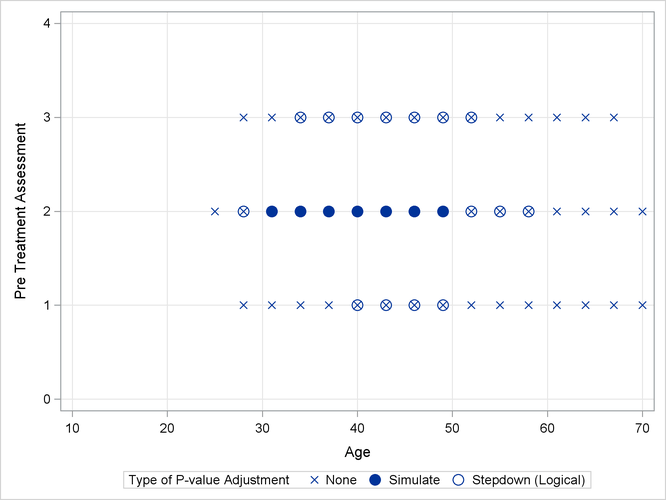
Output 43.13.2 shows a comparison of the significant comparisons (p < 0.05) based on unadjusted, adjusted, and step-down (TCTP) adjusted p-values. Clearly, the unadjusted results indicate the most significant results, but without protecting the Type I error rate for the group of tests. The adjusted p-values (filled circles) lead to a much smaller region in which the response surfaces between treatment and placebo are significantly different. The increased power of the TCTP procedure (open circles) over the standard multiplicity adjustment—without sacrificing Type I error protection—can be seen in the considerably larger region covered by the open circles.
The outcome variable in this clinical trial is an ordinal rating of patients in categories 0=terrible, 1=poor, 2=fair, 3=good, and 4=excellent. Furthermore, the observations from repeat visits for the same patients are likely correlated. The previous analysis removes the repeated measures aspect by defining efficacy as the average score at the final two visits. These averages are not normally distributed, however. The response surfaces for the two study arms can also be compared based on a model for ordinal data that takes correlation into account through random effects. Keeping with the theme of the previous analysis, the focus here for illustrative purposes is on the final two visits, and the pretreatment assessment score serves as a covariate in the model.
The following DATA step rearranges the data from the third and fourth on-treatment visits in univariate form with separate observations for the visits by patient:
data clinical_uv;
   set clinical;
   array time{2} t3-t4;
   do i=1 to 2; rating = time{i}; output; end;
run;
The basic model for the analysis is a proportional odds model with cumulative logit link (McCullagh, 1980) and J = 5 categories. In this model, separate intercepts (cutoffs) are modeled for the first ![]() cumulative categories and the intercepts are monotonically increasing. This guarantees ordering of the cumulative probabilities
and nonnegative category probabilities. Using the same covariate structure as in the previous analysis, the probability to
observe a rating in at most category
cumulative categories and the intercepts are monotonically increasing. This guarantees ordering of the cumulative probabilities
and nonnegative category probabilities. Using the same covariate structure as in the previous analysis, the probability to
observe a rating in at most category ![]() is
is
Because only the intercepts are dependent on the category, contrasts comparing regression coefficients can be formulated in
standard fashion. To accommodate the random and covariance structure of the repeated measures model, a random intercept ![]() is applied to the observations for each patient:
is applied to the observations for each patient:
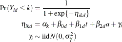
The shared random effect of the two observations creates a marginal correlation. Note that the random effects do not depend on category.
The following GLIMMIX statements fit this ordinal repeated measures model by maximum likelihood via the Laplace approximation and compute TCTP-adjusted p-values for the 105 estimates:
proc glimmix data=clinical_uv method=laplace;
   class center id drug;
   model rating = drug t0 age drug*age drug*t0 /
                  dist=multinomial link=cumlogit;
   random intercept / subject=id(center);
   covtest 0;
   estimate %contrast(10,70,3,1)
              / adjust=simulate(seed=1)
                stepdown(type=logical);
   ods output Estimates=EstStepDownMulti;
run;
The combination of DIST=MULTINOMIAL and LINK=CUMLOGIT requests the proportional odds model. The SUBJECT= effect nests patient IDs within centers, because patient IDs in the data set clinical are not unique within centers. (Specifying SUBJECT=ID*CENTER would have the same effect.) The COVTEST statement requests a likelihood ratio test for the significance of the random patient effect.
The estimate of the variance component for the random patient effect is substantial (Output 43.13.3), but so is its standard error.
Output 43.13.3: Model and Covariance Parameter Information
| Model Information | |
|---|---|
| Data Set | WORK.CLINICAL_UV |
| Response Variable | rating |
| Response Distribution | Multinomial (ordered) |
| Link Function | Cumulative Logit |
| Variance Function | Default |
| Variance Matrix Blocked By | ID(Center) |
| Estimation Technique | Maximum Likelihood |
| Likelihood Approximation | Laplace |
| Degrees of Freedom Method | Containment |
| Covariance Parameter Estimates | |||
|---|---|---|---|
| Cov Parm | Subject | Estimate | Standard Error |
| Intercept | ID(Center) | 10.3483 | 3.2599 |
| Tests of Covariance Parameters Based on the Likelihood |
|||||
|---|---|---|---|---|---|
| Label | DF | -2 Log Like | ChiSq | Pr > ChiSq | Note |
| Parameter list | 1 | 604.70 | 57.64 | <.0001 | MI |
| MI: P-value based on a mixture of chi-squares. |
The likelihood ratio test provides a better picture of the significance of the variance component. The difference in the –2 log likelihoods is 57.6, highly significant even if one does not apply the Self and Liang (1987) correction that halves the p-value in this instance.
The results for the 20 most significant estimates are requested with the following statements and shown in Output 43.13.4:
proc sort data=EstStepDownMulti;
   by Probt;
run;
proc print data=EstStepDownMulti(obs=20);
   var Label Estimate StdErr Probt AdjP;
run;
The p-values again show the “repeat” pattern corresponding to the monotonicity of the step-down procedure.
Output 43.13.4: The First 20 Estimates in the Ordinal Analysis
| Obs | Label | Estimate | StdErr | Probt | Adjp |
|---|---|---|---|---|---|
| 1 | 37 2 | -2.7224 | 0.8263 | 0.0013 | 0.0133 |
| 2 | 40 2 | -2.8857 | 0.8842 | 0.0015 | 0.0133 |
| 3 | 34 2 | -2.5590 | 0.7976 | 0.0018 | 0.0133 |
| 4 | 43 2 | -3.0491 | 0.9659 | 0.0021 | 0.0133 |
| 5 | 46 2 | -3.2124 | 1.0660 | 0.0032 | 0.0133 |
| 6 | 31 2 | -2.3957 | 0.8010 | 0.0034 | 0.0133 |
| 7 | 49 2 | -3.3758 | 1.1798 | 0.0051 | 0.0164 |
| 8 | 52 2 | -3.5391 | 1.3037 | 0.0077 | 0.0236 |
| 9 | 40 3 | -2.6263 | 0.9718 | 0.0080 | 0.0267 |
| 10 | 37 3 | -2.4630 | 0.9213 | 0.0087 | 0.0267 |
| 11 | 28 2 | -2.2323 | 0.8362 | 0.0088 | 0.0278 |
| 12 | 43 3 | -2.7897 | 1.0451 | 0.0088 | 0.0278 |
| 13 | 46 3 | -2.9530 | 1.1368 | 0.0107 | 0.0291 |
| 14 | 55 2 | -3.7025 | 1.4351 | 0.0112 | 0.0324 |
| 15 | 34 3 | -2.2996 | 0.8974 | 0.0118 | 0.0337 |
| 16 | 49 3 | -3.1164 | 1.2428 | 0.0136 | 0.0344 |
| 17 | 43 1 | -3.3085 | 1.3438 | 0.0154 | 0.0448 |
| 18 | 58 2 | -3.8658 | 1.5722 | 0.0155 | 0.0448 |
| 19 | 40 1 | -3.1451 | 1.2851 | 0.0160 | 0.0448 |
| 20 | 46 1 | -3.4718 | 1.4187 | 0.0160 | 0.0448 |
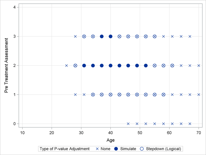
As previously, the comparisons were also performed with standard p-value adjustment via simulation. Output 43.13.5 displays the components of the regressor space in which the response surfaces differ significantly (p < 0.05) between the two treatment arms. As before, the most significant differences occur with unadjusted p-values at the cost of protecting only the individual Type I error rate. The standard multiplicity adjustment has considerably less power than the TCTP adjustment.