The GLIMMIX Procedure
-
Overview

-
Getting Started
-
SyntaxPROC GLIMMIX StatementBY StatementCLASS StatementCODE StatementCONTRAST StatementCOVTEST StatementEFFECT StatementESTIMATE StatementFREQ StatementID StatementLSMEANS StatementLSMESTIMATE StatementMODEL StatementNLOPTIONS StatementOUTPUT StatementPARMS StatementRANDOM StatementSLICE StatementSTORE StatementWEIGHT StatementProgramming StatementsUser-Defined Link or Variance Function
-
DetailsGeneralized Linear Models TheoryGeneralized Linear Mixed Models TheoryGLM Mode or GLMM ModeStatistical Inference for Covariance ParametersDegrees of Freedom MethodsEmpirical Covariance (Sandwich) EstimatorsExploring and Comparing Covariance MatricesProcessing by SubjectsRadial Smoothing Based on Mixed ModelsOdds and Odds Ratio EstimationParameterization of Generalized Linear Mixed ModelsResponse-Level Ordering and ReferencingComparing the GLIMMIX and MIXED ProceduresSingly or Doubly Iterative FittingDefault Estimation TechniquesDefault OutputNotes on Output StatisticsODS Table NamesODS Graphics
-
ExamplesBinomial Counts in Randomized BlocksMating Experiment with Crossed Random EffectsSmoothing Disease Rates; Standardized Mortality RatiosQuasi-likelihood Estimation for Proportions with Unknown DistributionJoint Modeling of Binary and Count DataRadial Smoothing of Repeated Measures DataIsotonic Contrasts for Ordered AlternativesAdjusted Covariance Matrices of Fixed EffectsTesting Equality of Covariance and Correlation MatricesMultiple Trends Correspond to Multiple Extrema in Profile LikelihoodsMaximum Likelihood in Proportional Odds Model with Random EffectsFitting a Marginal (GEE-Type) ModelResponse Surface Comparisons with Multiplicity AdjustmentsGeneralized Poisson Mixed Model for Overdispersed Count DataComparing Multiple B-SplinesDiallel Experiment with Multimember Random EffectsLinear Inference Based on Summary DataWeighted Multilevel Model for Survey Data
- References
Clayton and Kaldor (1987, Table 1) present data on observed and expected cases of lip cancer in the 56 counties of Scotland between 1975 and 1980. The expected number of cases was determined by a separate multiplicative model that accounted for the age distribution in the counties. The goal of the analysis is to estimate the county-specific log-relative risks, also known as standardized mortality ratios (SMR).
If ![]() is the number of incident cases in county i and
is the number of incident cases in county i and ![]() is the expected number of incident cases, then the ratio of observed to expected counts,
is the expected number of incident cases, then the ratio of observed to expected counts, ![]() , is the standardized mortality ratio. Clayton and Kaldor (1987) assume there exists a relative risk
, is the standardized mortality ratio. Clayton and Kaldor (1987) assume there exists a relative risk ![]() that is specific to each county and is a random variable. Conditional on
that is specific to each county and is a random variable. Conditional on ![]() , the observed counts are independent Poisson variables with mean
, the observed counts are independent Poisson variables with mean ![]() .
.
An elementary mixed model for ![]() specifies only a random intercept for each county, in addition to a fixed intercept. Breslow and Clayton (1993), in their analysis of these data, also provide a covariate that measures the percentage of employees in agriculture, fishing,
and forestry. The expanded model for the region-specific relative risk in Breslow and Clayton (1993) is
specifies only a random intercept for each county, in addition to a fixed intercept. Breslow and Clayton (1993), in their analysis of these data, also provide a covariate that measures the percentage of employees in agriculture, fishing,
and forestry. The expanded model for the region-specific relative risk in Breslow and Clayton (1993) is
where ![]() and
and ![]() are fixed effects, and the
are fixed effects, and the ![]() are county random effects.
are county random effects.
The following DATA step creates the data set lipcancer. The expected number of cases is based on the observed standardized mortality ratio for counties with lip cancer cases, and
based on the expected counts reported by Clayton and Kaldor (1987, Table 1) for the counties without cases. The sum of the expected counts then equals the sum of the observed counts.
data lipcancer;
   input county observed expected employment SMR;
   if (observed > 0) then expCount = 100*observed/SMR;
   else expCount = expected;
   datalines;
 1  9  1.4 16 652.2
 2 39  8.7 16 450.3
 3 11  3.0 10 361.8
 4  9  2.5 24 355.7
 5 15  4.3 10 352.1
 6  8  2.4 24 333.3
 7 26  8.1 10 320.6
 8  7  2.3  7 304.3
 9  6  2.0  7 303.0
10 20  6.6 16 301.7
11 13  4.4  7 295.5
12  5  1.8 16 279.3
13  3  1.1 10 277.8
14  8  3.3 24 241.7
15 17  7.8  7 216.8
16  9  4.6 16 197.8
17  2  1.1 10 186.9
18  7  4.2  7 167.5
19  9  5.5  7 162.7
20  7  4.4 10 157.7
21 16 10.5  7 153.0
22 31 22.7 16 136.7
23 11  8.8 10 125.4
24  7  5.6  7 124.6
25 19 15.5  1 122.8
26 15 12.5  1 120.1
27  7  6.0  7 115.9
28 10  9.0  7 111.6
29 16 14.4 10 111.3
30 11 10.2 10 107.8
31  5  4.8  7 105.3
32  3  2.9 24 104.2
33  7  7.0 10  99.6
34  8  8.5  7  93.8
35 11 12.3  7  89.3
36  9 10.1  0  89.1
37 11 12.7 10  86.8
38  8  9.4  1  85.6
39  6  7.2 16  83.3
40  4  5.3  0  75.9
41 10 18.8  1  53.3
42  8 15.8 16  50.7
43  2  4.3 16  46.3
44  6 14.6  0  41.0
45 19 50.7  1  37.5
46  3  8.2  7  36.6
47  2  5.6  1  35.8
48  3  9.3  1  32.1
49 28 88.7  0  31.6
50  6 19.6  1  30.6
51  1  3.4  1  29.1
52  1  3.6  0  27.6
53  1  5.7  1  17.4
54  1  7.0  1  14.2
55  0  4.2 16   0.0
56  0  1.8 10   0.0
;
Because the mean of the Poisson variates, conditional on the random effects, is ![]() , applying a log link yields
, applying a log link yields
The term ![]() is an offset, a regressor variable whose coefficient is known to be one. Note that it is assumed that the
is an offset, a regressor variable whose coefficient is known to be one. Note that it is assumed that the ![]() are known; they are not treated as random variables.
are known; they are not treated as random variables.
The following statements fit this model by residual pseudo-likelihood:
proc glimmix data=lipcancer;
   class county;
   x    = employment / 10;
   logn = log(expCount);
   model observed = x / dist=poisson offset=logn
                        solution ddfm=none;
   random county;
   SMR_pred = 100*exp(_zgamma_ + _xbeta_);
   id employment SMR SMR_pred;
   output out=glimmixout;
run;
The offset is created with the assignment statement
logn = log(expCount);
and is associated with the linear predictor through the OFFSET= option in the MODEL statement. The statement
x = employment / 10;
transforms the covariate measuring percentage of employment in agriculture, fisheries, and forestry to agree with the analysis
of Breslow and Clayton (1993). The DDFM=NONE option in the MODEL statement requests chi-square tests and z tests instead of the default F tests and t tests by setting the denominator degrees of freedom in tests of fixed effects to ![]() .
.
The statement
SMR_pred = 100*exp(_zgamma_ + _xbeta_);
calculates the fitted standardized mortality rate. Note that the offset variable does not contribute to the exponentiated term.
The OUTPUT statement saves results of the calculations to the output data set glimmixout. The ID statement specifies that only the listed variables are written to the output data set.
Output 43.3.1: Model Information in Poisson GLMM
| Model Information | |
|---|---|
| Data Set | WORK.LIPCANCER |
| Response Variable | observed |
| Response Distribution | Poisson |
| Link Function | Log |
| Variance Function | Default |
| Offset Variable | logn = log(expCount); |
| Variance Matrix | Not blocked |
| Estimation Technique | Residual PL |
| Degrees of Freedom Method | None |
| Class Level Information | ||
|---|---|---|
| Class | Levels | Values |
| county | 56 | 1 2 3 4 5 6 7 8 9 10 11 12 13 14 15 16 17 18 19 20 21 22 23 24 25 26 27 28 29 30 31 32 33 34 35 36 37 38 39 40 41 42 43 44 45 46 47 48 49 50 51 52 53 54 55 56 |
| Number of Observations Read | 56 |
|---|---|
| Number of Observations Used | 56 |
| Dimensions | |
|---|---|
| G-side Cov. Parameters | 1 |
| Columns in X | 2 |
| Columns in Z | 56 |
| Subjects (Blocks in V) | 1 |
| Max Obs per Subject | 56 |
The GLIMMIX procedure displays in the “Model Information” table that the
offset variable was computed with programming statements and the final assignment statement from your GLIMMIX statements (Output 43.3.1). There are two columns in the ![]() matrix, corresponding to the intercept and the regressor
matrix, corresponding to the intercept and the regressor ![]() . There are 56 columns in the
. There are 56 columns in the ![]() matrix, however, one for each observation in the data set (Output 43.3.1).
matrix, however, one for each observation in the data set (Output 43.3.1).
The optimization involves only a single covariance parameter, the variance of the county effect (Output 43.3.2). Because this parameter is a variance, the GLIMMIX procedure imposes a lower boundary constraint; the solution for the variance is bounded by zero from below.
Output 43.3.2: Optimization Information in Poisson GLMM
| Optimization Information | |
|---|---|
| Optimization Technique | Dual Quasi-Newton |
| Parameters in Optimization | 1 |
| Lower Boundaries | 1 |
| Upper Boundaries | 0 |
| Fixed Effects | Profiled |
| Starting From | Data |
Following the initial creation of pseudo-data and the fit of a linear mixed model, the procedure goes through five more updates of the pseudo-data, each associated with a separate optimization (Output 43.3.3). Although the objective function in each optimization is the negative of twice the restricted maximum likelihood for that pseudo-data, there is no guarantee that across the outer iterations the objective function decreases in subsequent optimizations. In this example, minus twice the residual maximum likelihood at convergence takes on its smallest value at the initial optimization and increases in subsequent optimizations.
Output 43.3.3: Iteration History in Poisson GLMM
| Iteration History | |||||
|---|---|---|---|---|---|
| Iteration | Restarts | Subiterations | Objective Function |
Change | Max Gradient |
| 0 | 0 | 4 | 123.64113992 | 0.20997891 | 3.848E-8 |
| 1 | 0 | 3 | 127.05866018 | 0.03393332 | 0.000048 |
| 2 | 0 | 2 | 127.48839749 | 0.00223427 | 5.753E-6 |
| 3 | 0 | 1 | 127.50502469 | 0.00006946 | 1.938E-7 |
| 4 | 0 | 1 | 127.50528068 | 0.00000118 | 1.09E-7 |
| 5 | 0 | 0 | 127.50528481 | 0.00000000 | 1.299E-6 |
| Convergence criterion (PCONV=1.11022E-8) satisfied. |
The “Covariance Parameter Estimates” table in Output 43.3.4 shows the estimate of the variance of the region-specific log-relative risks. There is significant county-to-county heterogeneity in risks. If the covariate were removed from the analysis, as in Clayton and Kaldor (1987), the heterogeneity in county-specific risks would increase. (The fitted SMRs in Table 6 of Breslow and Clayton (1993) were obtained without the covariate x in the model.)
Output 43.3.4: Estimated Covariance Parameters in Poisson GLMM
| Covariance Parameter Estimates | ||
|---|---|---|
| Cov Parm | Estimate | Standard Error |
| county | 0.3567 | 0.09869 |
The “Solutions for Fixed Effects” table displays the estimates of ![]() and
and ![]() along with their standard errors and test statistics (Output 43.3.5). Because of the DDFM=NONE option in the MODEL statement, PROC GLIMMIX assumes that the degrees of freedom for the t tests of
along with their standard errors and test statistics (Output 43.3.5). Because of the DDFM=NONE option in the MODEL statement, PROC GLIMMIX assumes that the degrees of freedom for the t tests of ![]() are infinite. The p-values correspond to probabilities under a standard normal distribution. The covariate measuring employment percentages in
agriculture, fisheries, and forestry is significant. This covariate might be a surrogate for the exposure to sunlight, an
important risk factor for lip cancer.
are infinite. The p-values correspond to probabilities under a standard normal distribution. The covariate measuring employment percentages in
agriculture, fisheries, and forestry is significant. This covariate might be a surrogate for the exposure to sunlight, an
important risk factor for lip cancer.
Output 43.3.5: Fixed-Effects Parameter Estimates in Poisson GLMM
| Solutions for Fixed Effects | |||||
|---|---|---|---|---|---|
| Effect | Estimate | Standard Error | DF | t Value | Pr > |t| |
| Intercept | -0.4406 | 0.1572 | Infty | -2.80 | 0.0051 |
| x | 0.6799 | 0.1409 | Infty | 4.82 | <.0001 |
You can examine the quality of the fit of this model with various residual plots. A panel of studentized residuals is requested with the following statements:
ods graphics on;
ods select StudentPanel;

proc glimmix data=lipcancer plots=studentpanel;
   class county;
   x    = employment / 10;
   logn = log(expCount);
   model observed = x / dist=poisson offset=logn s ddfm=none;
   random county;
run;

ods graphics off;
The graph in the upper-left corner of the panel displays studentized residuals plotted against the linear predictor (Output 43.3.6). The default of the GLIMMIX procedure is to use the estimated BLUPs in the construction of the residuals and to present them on the linear scale, which in this case is the logarithmic scale. You can change the type of the computed residual with the TYPE= suboptions of each paneled display. For example, the option PLOTS=STUDENTPANEL(TYPE=NOBLUP) would request a paneled display of the marginal residuals on the linear scale.
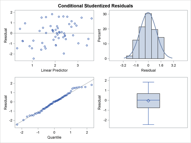
The graph in the upper-right corner of the panel shows a histogram with overlaid normal density. A Q-Q plot and a box plot are shown in the lower cells of the panel.
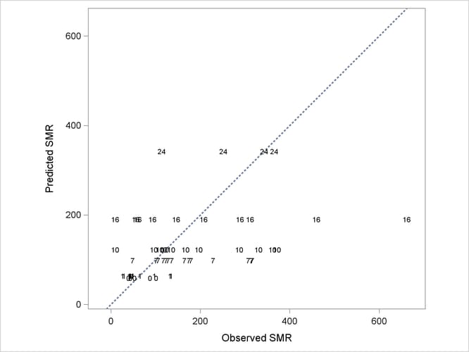
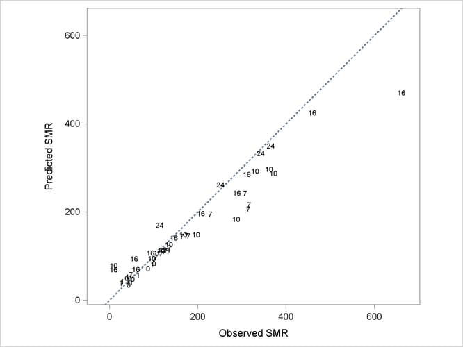
The following statements produce a graph of the observed and predicted standardized mortality ratios (Output 43.3.7):
proc template;
   define statgraph scatter;
      BeginGraph;
         layout overlayequated / yaxisopts=(label='Predicted SMR')
                                 xaxisopts=(label='Observed SMR')
                                 equatetype=square;
            lineparm y=0 slope=1 x=0 /
                   lineattrs = GraphFit(pattern=dash)
                   extend    = true;
            scatterplot y=SMR_pred x=SMR /
                    markercharacter = employment;
         endlayout;
      EndGraph;
   end;
run;
proc sgrender data=glimmixout template=scatter;
run;
In Output 43.3.7, fitted SMRs tend to be larger than the observed SMRs for counties with small observed SMR and smaller than the observed SMRs for counties with high observed SMR.
To demonstrate the impact of the random effects adjustment to the log-relative risks, the following statements fit a Poisson regression model (a GLM) by maximum likelihood:
proc glimmix data=lipcancer;
   x    = employment / 10;
   logn = log(expCount);
   model observed = x / dist=poisson offset=logn
                        solution ddfm=none;
   SMR_pred = 100*exp(_zgamma_ + _xbeta_);
   id employment SMR SMR_pred;
   output out=glimmixout;
run;
The GLIMMIX procedure defaults to maximum likelihood estimation because these statements fit a generalized linear model with nonnormal distribution. As a consequence, the SMRs are county specific only to the extent that the risks vary with the value of the covariate. But risks are no longer adjusted based on county-to-county heterogeneity in the observed incidence count.
Because of the absence of random effects, the GLIMMIX procedure recognizes the model as a generalized linear model and fits it by maximum likelihood (Output 43.3.8). The variance matrix is diagonal because the observations are uncorrelated.
Output 43.3.8: Model Information in Poisson GLM
| Model Information | |
|---|---|
| Data Set | WORK.LIPCANCER |
| Response Variable | observed |
| Response Distribution | Poisson |
| Link Function | Log |
| Variance Function | Default |
| Offset Variable | logn = log(expCount); |
| Variance Matrix | Diagonal |
| Estimation Technique | Maximum Likelihood |
| Degrees of Freedom Method | None |
The “Dimensions” table shows that there are no G-side random effects in this model and no R-side scale parameter either (Output 43.3.9).
Output 43.3.9: Model Dimensions Information in Poisson GLM
| Dimensions | |
|---|---|
| Columns in X | 2 |
| Columns in Z | 0 |
| Subjects (Blocks in V) | 1 |
| Max Obs per Subject | 56 |
Because this is a GLM, the GLIMMIX procedure defaults to the Newton-Raphson algorithm, and the fixed effects (intercept and slope) comprise the parameters in the optimization (Output 43.3.10). (The default optimization technique for a GLM is the Newton-Raphson method.)
Output 43.3.10: Optimization Information in Poisson GLM
| Optimization Information | |
|---|---|
| Optimization Technique | Newton-Raphson |
| Parameters in Optimization | 2 |
| Lower Boundaries | 0 |
| Upper Boundaries | 0 |
| Fixed Effects | Not Profiled |
The estimates of ![]() and
and ![]() have changed from the previous analysis. In the GLMM, the estimates were
have changed from the previous analysis. In the GLMM, the estimates were ![]() and
and ![]() (Output 43.3.11).
(Output 43.3.11).
Output 43.3.11: Parameter Estimates in Poisson GLM
| Parameter Estimates | |||||
|---|---|---|---|---|---|
| Effect | Estimate | Standard Error | DF | t Value | Pr > |t| |
| Intercept | -0.5419 | 0.06951 | Infty | -7.80 | <.0001 |
| x | 0.7374 | 0.05954 | Infty | 12.38 | <.0001 |
More importantly, without the county-specific adjustments through the best linear unbiased predictors of the random effects, the predicted SMRs are the same for all counties with the same percentage of employees in agriculture, fisheries, and forestry (Output 43.3.12).