The GLIMMIX Procedure
-
Overview

-
Getting Started
-
SyntaxPROC GLIMMIX StatementBY StatementCLASS StatementCODE StatementCONTRAST StatementCOVTEST StatementEFFECT StatementESTIMATE StatementFREQ StatementID StatementLSMEANS StatementLSMESTIMATE StatementMODEL StatementNLOPTIONS StatementOUTPUT StatementPARMS StatementRANDOM StatementSLICE StatementSTORE StatementWEIGHT StatementProgramming StatementsUser-Defined Link or Variance Function
-
DetailsGeneralized Linear Models TheoryGeneralized Linear Mixed Models TheoryGLM Mode or GLMM ModeStatistical Inference for Covariance ParametersDegrees of Freedom MethodsEmpirical Covariance (Sandwich) EstimatorsExploring and Comparing Covariance MatricesProcessing by SubjectsRadial Smoothing Based on Mixed ModelsOdds and Odds Ratio EstimationParameterization of Generalized Linear Mixed ModelsResponse-Level Ordering and ReferencingComparing the GLIMMIX and MIXED ProceduresSingly or Doubly Iterative FittingDefault Estimation TechniquesDefault OutputNotes on Output StatisticsODS Table NamesODS Graphics
-
ExamplesBinomial Counts in Randomized BlocksMating Experiment with Crossed Random EffectsSmoothing Disease Rates; Standardized Mortality RatiosQuasi-likelihood Estimation for Proportions with Unknown DistributionJoint Modeling of Binary and Count DataRadial Smoothing of Repeated Measures DataIsotonic Contrasts for Ordered AlternativesAdjusted Covariance Matrices of Fixed EffectsTesting Equality of Covariance and Correlation MatricesMultiple Trends Correspond to Multiple Extrema in Profile LikelihoodsMaximum Likelihood in Proportional Odds Model with Random EffectsFitting a Marginal (GEE-Type) ModelResponse Surface Comparisons with Multiplicity AdjustmentsGeneralized Poisson Mixed Model for Overdispersed Count DataComparing Multiple B-SplinesDiallel Experiment with Multimember Random EffectsLinear Inference Based on Summary DataWeighted Multilevel Model for Survey Data
- References
- ALPHA=number
-
requests that a t-type confidence interval be constructed for each of the fixed-effects parameters with confidence level 1 – number. The value of number must be between 0 and 1; the default is 0.05.
- CHISQ
-
requests that chi-square tests be performed for all specified effects in addition to the F tests. Type III tests are the default; you can produce the Type I and Type II tests by using the HTYPE= option.
- CL
-
requests that t-type confidence limits be constructed for each of the fixed-effects parameter estimates. The confidence level is 0.95 by default; this can be changed with the ALPHA= option.
- CORRB
-
produces the correlation matrix from the approximate covariance matrix of the fixed-effects parameter estimates.
- COVB<(DETAILS)>
-
produces the approximate variance-covariance matrix of the fixed-effects parameter estimates
 . In a generalized linear mixed model this matrix typically takes the form
  and can be obtained by sweeping the mixed model equations; see the section Estimated Precision of Estimates. In a model without random effects, it is obtained from the inverse of the observed or expected Hessian matrix. Which Hessian
is used in the computation depends on whether the procedure is in scoring mode (see the SCORING= option in the PROC GLIMMIX statement) and whether the EXPHESSIAN option is in effect. Note that if you use EMPIRICAL= or DDFM=KENWARDROGER, the matrix displayed by the COVB option is the empirical (sandwich) estimator or the adjusted estimator, respectively.
and can be obtained by sweeping the mixed model equations; see the section Estimated Precision of Estimates. In a model without random effects, it is obtained from the inverse of the observed or expected Hessian matrix. Which Hessian
is used in the computation depends on whether the procedure is in scoring mode (see the SCORING= option in the PROC GLIMMIX statement) and whether the EXPHESSIAN option is in effect. Note that if you use EMPIRICAL= or DDFM=KENWARDROGER, the matrix displayed by the COVB option is the empirical (sandwich) estimator or the adjusted estimator, respectively.
The DETAILS suboption of the COVB option enables you to obtain a table of statistics about the covariance matrix of the fixed effects. If an adjusted estimator is used because of the EMPIRICAL= or DDFM=KENWARDROGER option, the GLIMMIX procedure displays statistics for the adjusted and unadjusted estimators as well as statistics comparing them. This enables you to diagnose, for example, changes in rank (because of an insufficient number of subjects for the empirical estimator) and to assess the extent of the covariance adjustment. In addition, the GLIMMIX procedure then displays the unadjusted (=model-based) covariance matrix of the fixed-effects parameter estimates. For more details, see the section Exploring and Comparing Covariance Matrices.
- COVBI
-
produces the inverse of the approximate covariance matrix of the fixed-effects parameter estimates.
-
DDF=value-list
DF=value-list -
enables you to specify your own denominator degrees of freedom for the fixed effects. The value-list specification is a list of numbers or missing values (.) separated by commas. The degrees of freedom should be listed in the order in which the effects appear in the “Type III Tests of Fixed Effects” table. If you want to retain the default degrees of freedom for a particular effect, use a missing value for its location in the list. For example, the statement assigns 3 denominator degrees of freedom to
Aand 4.7 toA*B, while those forBremain the same:model Y = A B A*B / ddf=3,.,4.7;
If you select a degrees-of-freedom method with the DDFM= option, then nonmissing, positive values in value-list override the degrees of freedom for the particular effect. For example, the statement assigns 3 and 6 denominator degrees of freedom in the test of the
Amain effect and theA*Binteraction, respectively:model Y = A B A*B / ddf=3,.,6 ddfm=Satterth;
The denominator degrees of freedom for the test for the
Beffect are determined from a Satterthwaite approximation.Note that the DDF= and DDFM= options determine the degrees of freedom in the “Type I Tests of Fixed Effects,” “Type II Tests of Fixed Effects,” and “Type III Tests of Fixed Effects” tables. These degrees of freedom are also used in determining the degrees of freedom in tests and confidence intervals from the CONTRAST, ESTIMATE, LSMEANS, and LSMESTIMATE statements. Exceptions from this rule are noted in the documentation for the respective statements.
- DDFM=method
-
specifies the method for computing the denominator degrees of freedom for the tests of fixed effects that result from the MODEL, CONTRAST, ESTIMATE, LSMEANS, and LSMESTIMATE statements.
You can specify the following methods:
-
BETWITHIN
BW -
assigns within-subject degrees of freedom to a fixed effect if the fixed effect changes within a subject, and between-subject degrees of freedom otherwise. This method is the default for models with only R-side random effects and a SUBJECT= option. Computational details can be found in the section Degrees of Freedom Methods.
-
CONTAIN
CON -
invokes the containment method to compute denominator degrees of freedom. This method is the default when the model contains G-side random effects. Computational details can be found in the section Degrees of Freedom Methods.
-
KENWARDROGER<(FIRSTORDER)>
KENROGER<(FIRSTORDER)>
KR<(FIRSTORDER)> -
applies the (prediction) standard error and degrees-of-freedom correction detailed by Kenward and Roger (1997). This approximation involves adjusting the estimated variance-covariance matrix of the fixed and random effects in a manner similar to that of Prasad and Rao (1990); Harville and Jeske (1992); Kackar and Harville (1984). Satterthwaite-type degrees of freedom are then computed based on this adjustment. Computational details can be found in the section Degrees of Freedom Methods.
-
KENWARDROGER2
KENROGER2
KR2 -
applies the (prediction) standard error and degrees-of-freedom correction that are detailed by Kenward and Roger (2009). This correction further reduces the precision estimator bias for the fixed and random effects under nonlinear covariance structures. Computational details can be found in the section Degrees of Freedom Methods.
- NONE
-
specifies that no denominator degrees of freedom be applied. PROC GLIMMIX then essentially assumes that infinite degrees of freedom are available in the calculation of p-values. The p-values for t tests are then identical to p-values that are derived from the standard normal distribution. In the case of F tests, the p-values are equal to those of chi-square tests that are determined as follows: if
 is the observed value of the F test with l numerator degrees of freedom, then
![\[ p = \mr {Pr}\{ F_{l,\infty } > F_{\mathit{obs}} \} = \mr {Pr}\{ \chi ^2_ l > l F_{\mathit{obs}} \} \]](images/statug_glimmix0227.png)
Regardless of the DDFM= method, you can obtain these chi-square p-values with the CHISQ option in the MODEL statement.
-
RESIDUAL
RES -
performs all tests by using the residual degrees of freedom,
 , where n is the sum of the frequencies of observations or the sum of frequencies of event/trials pairs. This method is the default degrees of freedom method for GLMs and overdispersed GLMs.
-
SATTERTHWAITE
SAT -
performs a general Satterthwaite approximation for the denominator degrees of freedom in a generalized linear mixed model. This method is a generalization of the techniques that are described in Giesbrecht and Burns (1985); McLean and Sanders (1988); Fai and Cornelius (1996). The method can also include estimated random effects. Computational details can be found in the section Degrees of Freedom Methods.
When the asymptotic variance matrix of the covariance parameters is found to be singular, a generalized inverse is used. Covariance parameters with zero variance then do not contribute to the degrees of freedom adjustment for DDFM=SATTERTH and DDFM=KENWARDROGER, and a message is written to the log.
-
BETWITHIN
-
DISTRIBUTION=keyword
DIST=keyword
D=keyword
ERROR=keyword
E=keyword -
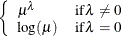
specifies the built-in (conditional) probability distribution of the data. If you specify the DIST= option and you do not specify a user-defined link function, a default link function is chosen according to the following table. If you do not specify a distribution, the GLIMMIX procedure defaults to the normal distribution for continuous response variables and to the multinomial distribution for classification or character variables, unless the events/trial syntax is used in the MODEL statement. If you choose the events/trial syntax, the GLIMMIX procedure defaults to the binomial distribution.
Table 43.12 lists the values of the DIST= option and the corresponding default link functions. For the case of generalized linear models with these distributions, you can find expressions for the log-likelihood functions in the section Maximum Likelihood.
Table 43.12: Keyword Values of the DIST= Option
Default Link
Numeric
DIST=
Distribution
Function
Value
BETA
beta
logit
12
BINARY
binary
logit
4
BINOMIAL | BIN | B
binomial
logit
3
EXPONENTIAL | EXPO
exponential
log
9
GAMMA | GAM
gamma
log
5
GAUSSIAN | G | NORMAL | N
normal
identity
1
GEOMETRIC | GEOM
geometric
log
8
INVGAUSS | IGAUSSIAN | IG
inverse Gaussian
inverse squared
6
(power(–2) )
LOGNORMAL | LOGN
lognormal
identity
11
MULTINOMIAL | MULTI | MULT
multinomial
cumulative logit
NA
NEGBINOMIAL | NEGBIN | NB
negative binomial
log
7
POISSON | POI | P
Poisson
log
2
TCENTRAL | TDIST | T
t
identity
10
BYOBS(variable)
multivariate
varied
NA
Note that the PROC GLIMMIX default link for the gamma or exponential distribution is not the canonical link (the reciprocal link).
The numeric value in the last column of Table 43.12 can be used in combination with DIST=BYOBS. The BYOBS(variable) syntax designates a variable whose value identifies the distribution to which an observation belongs. If the variable is numeric, its values must match values in the last column of Table 43.12. If the variable is not numeric, an observation’s distribution is identified by the first four characters of the distribution’s name in the leftmost column of the table. Distributions whose numeric value is “NA” cannot be used with DIST=BYOBS.
If the variable in BYOBS(variable) is a data set variable, it can also be used in the CLASS statement of the GLIMMIX procedure. For example, this provides a convenient method to model multivariate data jointly while varying fixed-effects components across outcomes. Assume that, for example, for each patient, a count and a continuous outcome were observed; the count data are modeled as Poisson data and the continuous data are modeled as gamma variates. The following statements fit a Poisson and a gamma regression model simultaneously:
proc sort data=yourdata;
   by patient;
run;
data yourdata;
   set yourdata;
   by patient;
   if first.patient then dist='POIS' else dist='GAMM';
run;
proc glimmix data=yourdata;
   class treatment dist;
   model y = dist treatment*dist / dist=byobs(dist);
run;
The two models have separate intercepts and treatment effects. To correlate the outcomes, you can share a random effect between the observations from the same patient:
proc glimmix data=yourdata;
   class treatment dist patient;
   model y = dist treatment*dist / dist=byobs(dist);
   random intercept / subject=patient;
run;
Or, you could use an R-side correlation structure:
proc glimmix data=yourdata;
   class treatment dist patient;
   model y = dist treatment*dist / dist=byobs(dist);
   random _residual_ / subject=patient type=un;
run;
Although DIST=BYOBS(variable) is used to model multivariate data, you only need a single response variable in PROC GLIMMIX. The responses are in “univariate” form. This allows, for example, different missing value patterns across the responses. It does, however, require that all response variables be numeric.
The default links that are assigned when DIST=BYOBS is in effect correspond to the respective default links in Table 43.12.
When you choose DIST=LOGNORMAL, the GLIMMIX procedure models the logarithm of the response variable as a normal random variable. That is, the mean and variance are estimated on the logarithmic scale, assuming a normal distribution,
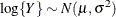 . This enables you to draw on options that require a distribution in the exponential family—for example, by using a scoring
algorithm in a GLM. To convert means and variances for
. This enables you to draw on options that require a distribution in the exponential family—for example, by using a scoring
algorithm in a GLM. To convert means and variances for  into those of Y, use the relationships
![\begin{align*} \mr {E}[Y] & = \exp \{ \mu \} \sqrt {\omega } \\ \mr {Var}[Y] & = \exp \{ 2\mu \} \omega (\omega -1) \\ \omega & = \exp \{ \sigma ^2\} \end{align*}](images/statug_glimmix0231.png)
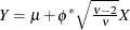
The DIST=T option models the data as a shifted and scaled central t variable. This enables you to model data with heavy-tailed distributions. If Y denotes the response and X has a
 distribution with
  degrees of freedom, then PROC GLIMMIX models
![\[ Y = \mu + \sqrt {\phi } X \]](images/statug_glimmix0233.png)
In this parameterization, Y has mean
 and variance
  .
.
By default,
 . You can supply different degrees of freedom for the t variate as in the following statements:
proc glimmix;
   class a b;
   model y = b x b*x / dist=tcentral(9.6);
   random a;
run;
The GLIMMIX procedure does not accept values for the degrees of freedom parameter less than 3.0. If the t distribution is used with the DIST=BYOBS(variable) specification, the degrees of freedom are fixed at
 . For mixed models where parameters are estimated based on linearization, choosing DIST=T instead of DIST=NORMAL affects only
the residual variance, which decreases by the factor
. For mixed models where parameters are estimated based on linearization, choosing DIST=T instead of DIST=NORMAL affects only
the residual variance, which decreases by the factor  .
.
Note that in SAS 9.1, the GLIMMIX procedure modeled
 . The scale parameter of the parameterizations are related as
 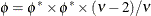 .
.
The DIST=BETA option implements the parameterization of the beta distribution in Ferrari and Cribari-Neto (2004). If Y has a
 density, so that
 ![$\mr {E}[Y] = \mu = \alpha /(\alpha +\beta )$](images/statug_glimmix0241.png) , this parameterization uses the variance function
, this parameterization uses the variance function 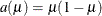 and
and ![$\mr {Var}[Y] = a(\mu )/(1+\phi )$](images/statug_glimmix0243.png) .
.
See the section Maximum Likelihood for the log likelihoods of the distributions fitted by the GLIMMIX procedure.
- E
-
requests that Type I, Type II, and Type III
 matrix coefficients
be displayed for all specified effects.
matrix coefficients
be displayed for all specified effects.
- E1 | EI
-
requests that Type I
matrix coefficients
be displayed for all specified effects.
- E2 | EII
-
requests that Type II
matrix coefficients
be displayed for all specified effects.
- E3 | EIII
-
requests that Type III
matrix coefficients
be displayed for all specified effects.
- HTYPE=value-list
-
indicates the type of hypothesis test to perform on the fixed effects. Valid entries for values in the value-list are 1, 2, and 3, corresponding to Type I, Type II, and Type III tests. The default value is 3. You can specify several types by separating the values with a comma or a space. The ODS table names are “Tests1,” “Tests2,” and “Tests3” for the Type I, Type II, and Type III tests, respectively.
- INTERCEPT
-
adds a row to the tables for Type I, II, and III tests corresponding to the overall intercept.
- LINK=keyword
-
specifies the link function in the generalized linear mixed model. The keywords and their associated built-in link functions are shown in Table 43.13.
Table 43.13: Built-in Link Functions of the GLIMMIX Procedure
Link
Numeric
LINK=
Function

Value
CUMCLL | CCLL
cumulative
NA
complementary log-log
CUMLOGIT | CLOGIT
cumulative logit

NA
CUMLOGLOG
cumulative log-log

NA
CUMPROBIT | CPROBIT
cumulative probit

NA
CLOGLOG | CLL
complementary log-log
5
GLOGIT | GENLOGIT
generalized logit
NA
IDENTITY | ID
identity
1
LOG
log

4
LOGIT
logit

2
LOGLOG
log-log

6
PROBIT
probit

3
POWER(
 ) | POW()
power with exponent
= number
NA
POWERMINUS2
power with exponent -2

8
RECIPROCAL | INVERSE
reciprocal

7
BYOBS(variable)
varied
varied
NA
For the probit and cumulative probit links,
 denotes the quantile function of the standard normal distribution. For the other cumulative links,
  denotes a cumulative category probability. The cumulative and generalized logit link functions are appropriate only for the
multinomial distribution. When you choose a cumulative link function, PROC GLIMMIX assumes that the data are ordinal. When
you specify LINK=GLOGIT, the GLIMMIX procedure assumes that the data are nominal (not ordered).
denotes a cumulative category probability. The cumulative and generalized logit link functions are appropriate only for the
multinomial distribution. When you choose a cumulative link function, PROC GLIMMIX assumes that the data are ordinal. When
you specify LINK=GLOGIT, the GLIMMIX procedure assumes that the data are nominal (not ordered).
The numeric value in the rightmost column of Table 43.13 can be used in conjunction with LINK=BYOBS(variable). This syntax designates a variable whose values identify the link function associated with an observation. If the variable is numeric, its values must match those in the last column of Table 43.13. If the variable is not numeric, an observation’s link function is determined by the first four characters of the link’s name in the first column. Those link functions whose numeric value is “NA” cannot be used with LINK=BYOBS(variable).
You can define your own link function through programming statements. See the section User-Defined Link or Variance Function for more information about how to specify a link function. If a user-defined link function is in effect, the specification in the LINK= option is ignored. If you specify neither the LINK= option nor a user-defined link function, then the default link function is chosen according to Table 43.12.
-
LWEIGHT=FIRSTORDER | FIRO
LWEIGHT=NONE
LWEIGHT=VAR -
determines how weights are used in constructing the coefficients for Type I through Type III
matrices. The default is LWEIGHT=VAR, and the values of the WEIGHT variable are used in forming crossproduct matrices. If you specify LWEIGHT=FIRO, the weights incorporate the WEIGHT variable
as well as the first-order weights of the linearized model. For LWEIGHT=NONE, the  matrix coefficients are based on the raw crossproduct matrix, whether a WEIGHT variable is specified or not.
- NOCENTER
-
requests that the columns of the
 matrix are not centered and
scaled. By default, the columns of are centered and scaled. Unless the NOCENTER option is in effect, is replaced by
matrix are not centered and
scaled. By default, the columns of are centered and scaled. Unless the NOCENTER option is in effect, is replaced by  during estimation. The columns of are computed as follows:
-
In models with an intercept, the intercept column remains the same and the jth entry in row i of
is
![\[ x^*_{ij} = \frac{x_{ij}-\overline{x}_ j}{\sqrt {\sum _{i=1}^{n}(x_{ij}-\overline{x}_ j)^2}} \]](images/statug_glimmix0260.png)
-
In models without intercept, no centering takes place and the jth entry in row i of
is
![\[ x^*_{ij} = \frac{x_{ij}}{\sqrt {\sum _{i=1}^{n}(x_{ij}-\overline{x}_ j)^2}} \]](images/statug_glimmix0261.png)
The effects of centering and scaling are removed when results are reported. For example, if the covariance matrix of the fixed effects is printed with the COVB option of the MODEL statement, the covariances are reported in terms of the original parameters, not the centered and scaled versions. If you specify the STDCOEF option, fixed-effects parameter estimates and their standard errors are reported in terms of the standardized (scaled and/or centered) coefficients in addition to the usual results in noncentered form.
-
- NOINT
-
requests that no intercept be included in the fixed-effects model. An intercept is included by default.
-
ODDSRATIO<(odds-ratio-options)>
OR<(odds-ratio-options)> -
requests estimates of odds ratios and their confidence limits, provided the link function is the logit, cumulative logit, or generalized logit. Odds ratios are produced for the following:
-
classification main effects, if they appear in the MODEL statement
-
continuous variables in the MODEL statement, unless they appear in an interaction with a classification effect
-
continuous variables in the MODEL statement at fixed levels of a classification effect, if the MODEL statement contains an interaction of the two
-
continuous variables in the MODEL statement, if they interact with other continuous variables
You can specify the following odds-ratio-options to create customized odds ratio results.
- AT var-list=value-list
-
specifies the reference values for continuous variables in the model. By default, the average value serves as the reference. Consider, for example, the following statements:
proc glimmix;
   class A;
   model y = A x A*x / dist=binary oddsratio;
run;
Odds ratios for
Aare based on differences of least squares means for whichxis set to its mean. Odds ratios forxare computed by differencing two sets of least squares mean for theAfactor. One set is computed atx= , and the second set is computed at
 x= . The following MODEL statement changes the reference value for
 xto 3:model y = A x A*x / dist=binary oddsratio(at x=3); - DIFF<=difftype>
-
controls the type of differences for classification main effects. By default, odds ratios compare the odds of a response for level j of a factor to the odds of the response for the last level of that factor (DIFF=LAST). The DIFF=FIRST option compares the levels against the first level, DIFF=ALL produces odds ratios based on all pairwise differences, and DIFF=NONE suppresses odds ratios for classification main effects.
- LABEL
-
displays a label in the “Odds Ratio Estimates” table. The table describes the comparison associated with the table row.
- UNIT var-list=value-list
-
specifies the units in which the effects of continuous variable in the model are assessed. By default, odds ratios are computed for a change of one unit from the average. Consider a model with a classification factor
Awith 4 levels. The following statements produce an “Odds Ratio Estimates” table with 10 rows:proc glimmix; class A; model y = A x A*x / dist=binary oddsratio(diff=all unit x=2); run;The first
 rows correspond to pairwise differences of levels of
 A. The underlying log odds ratios are computed as differences ofAleast squares means. In the least squares mean computation the covariatexis set to. The next four rows compare least squares means for Aatx= and at
 x=. You can combine the AT and UNIT options to produce custom odds ratios. For example, the following statements produce an
“Odds Ratio Estimates” table with 8 rows:
proc glimmix;
   class A;
   model y = A x x*z / dist=binary
                       oddsratio(diff=all
                                 at   x   = 3
                                 unit x z = 2 4);
run;
The first
 rows correspond to pairwise differences of levels of
 A. The underlying log odds ratios are computed as differences ofAleast squares means. In the least squares mean computation, the covariatexis set to 3, and the covariatex*zis set to . The next odds ratio measures the effect of a change in
 x. It is based on differencing the linear predictor forx= and
and x*z= with the linear predictor for
 x= 3 andx*z=. The last odds ratio expresses a change in zby contrasting the linear predictors based onx= 3 andx*z= with the predictor based on
 x= 3 andx*z=.
To compute odds and odds ratios for general estimable functions and least squares means, see the ODDSRATIO option in the LSMEANS statement and the EXP options in the ESTIMATE and LSMESTIMATE statements.
For important details concerning interpretation and computation of odds ratios with the GLIMMIX procedure, see the section Odds and Odds Ratio Estimation.
-
- OFFSET=variable
-
specifies a variable to be used as an offset for the linear predictor. An offset plays the role of a fixed effect whose coefficient is known to be 1. You can use an offset in a Poisson model, for example, when counts have been obtained in time intervals of different lengths. With a log link function, you can model the counts as Poisson variables with the logarithm of the time interval as the offset variable. The offset variable cannot appear in the CLASS statement or elsewhere in the MODEL or RANDOM statement.
- REFLINP=r
-
specifies a value for the linear predictor of the reference level in the generalized logit model for nominal data. By default r=0.
-
SOLUTION
S -
requests that a solution for the fixed-effects parameters be produced. Using notation from the section Notation for the Generalized Linear Mixed Model, the fixed-effects parameter estimates are
, and their (approximate) estimated standard errors are the square roots of the diagonal elements of ![$\widehat{\mr {Var}}[\widehat{\bbeta }]$](images/statug_glimmix0271.png) . This matrix commonly is of the form
. This matrix commonly is of the form  in GLMMs. You can output this approximate variance matrix with the COVB option. See the section Details: GLIMMIX Procedure on the construction of
  in the various models.
Along with the estimates and their approximate standard errors, a t statistic is computed as the estimate divided by its standard error. The degrees of freedom for this t statistic matches the one appearing in the “Type III Tests of Fixed Effects” table under the effect containing the parameter. If DDFM=KENWARDROGER or DDFM=SATTERTHWAITE, the degrees of freedom are computed separately for each fixed-effect estimate, unless you override the value for any specific effect with the DDF=value-list option. The “Pr > |t|” column contains the two-tailed p-value corresponding to the t statistic and associated degrees of freedom. You can use the CL option to request confidence intervals for the fixed-effects parameters; they are constructed around the estimate by using a radius of the standard error times a percentage point from the t distribution.
- STDCOEF
-
reports solutions for fixed effects in terms of the standardized (scaled and/or centered) coefficients. This option has no effect when the NOCENTER option is specified or in models for multinomial data.
-
OBSWEIGHT<=variable>
OBSWT<=variable> -
specifies a variable to be used as the weight for the observation-level unit in a weighted multilevel model. If a weight variable is not specified in the OBSWEIGHT option, a weight of 1 is used. For details on the use of weights in multilevel models, see the section Pseudo-likelihood Estimation for Weighted Multilevel Models.
- ZETA=number
-
tunes the sensitivity in forming Type III functions. Any element in the estimable function basis with an absolute value less than number is set to 0. The default is 1E–8.